Code
smooth.spline(x, y, lambda)We observe \(y_i\) at each location \(x_i,\) for \(i=1,\ldots, n\). We imagine that the \(y\)’s are noisy versions of a smooth function, say \(f(\cdot)\), where the errors follow a normal distribution with constant variance. That is \[ y_i = f(x_i) + \epsilon_i, \quad \epsilon_i \sim \mathrm{N}(0,\sigma^2), \] for \(i=1,\ldots,n\), where \(f\) is smooth, the \(\epsilon_i\) are i.i.d., and \(f\) and \(\sigma^2\) are unknown. The log-likelihood for this situation is: \[ l(f; \mathbf{y}) = -\frac{1}{2\sigma^2} \sum_{i=1}^n \left(y_i - f(x_i)\right)^2 - n \log \sigma \tag{12.1}\] and we wish to estimate \(f\) for a given data set \(\mathbf{y}=\{y_1,\dots, y_n\}\). With no constraints on \(f\), the log-likelihood would be maximised by setting \(f(x_i)=y_i\) for all \(i\), and we would estimate the noise variance as \(\hat{\sigma}^2=0\). This takes no account of randomness in the data and \(f\) would in general need to be quite wiggly to achieve this fit.
Figure 12.1 (a) shows such an interpolation of noisy data. This would be of little use for explanation, interpolation or prediction.
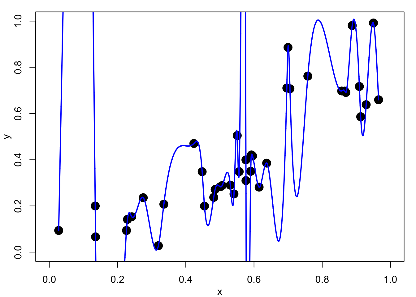
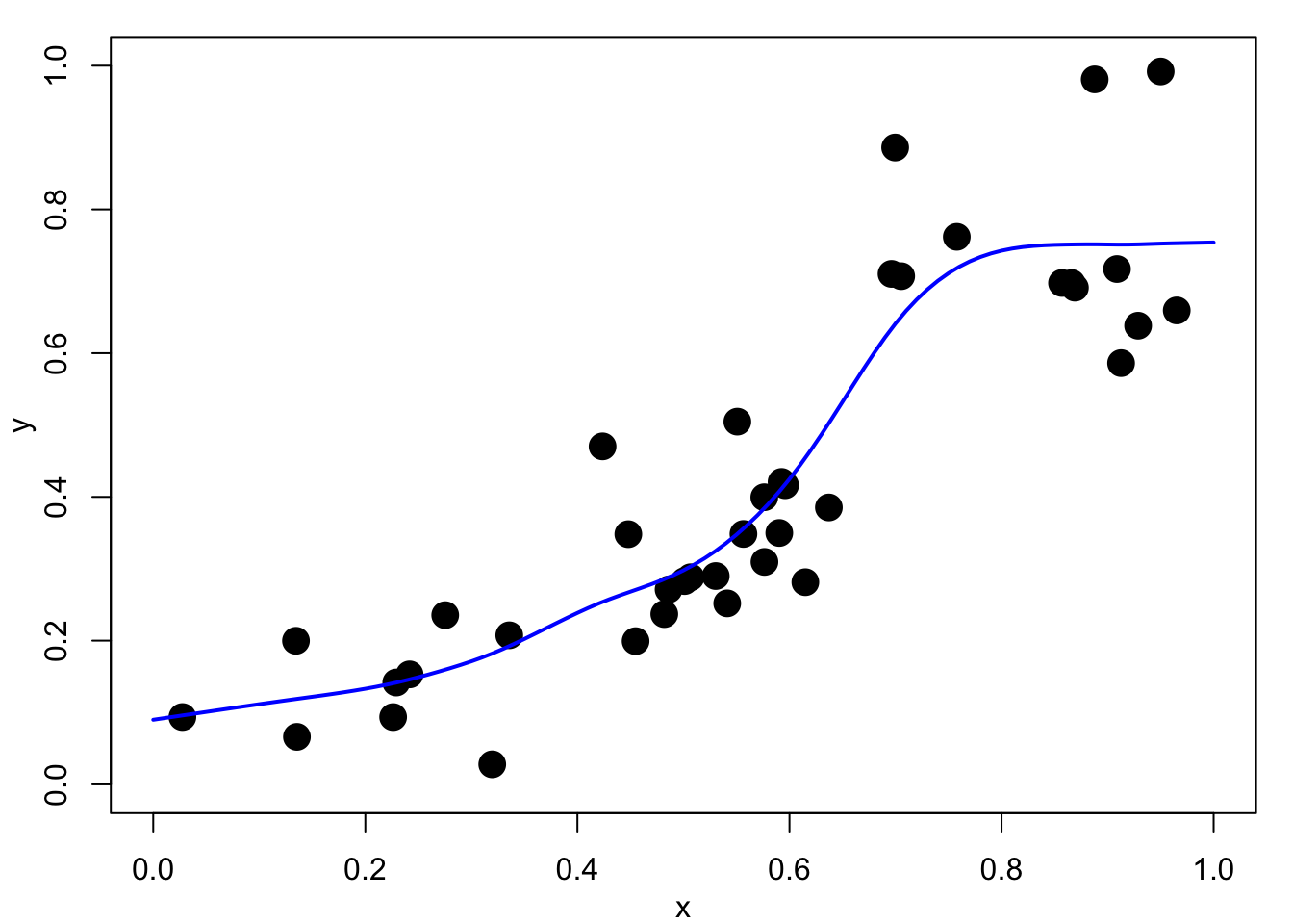
We do not expect, or even want, the fitted function \(f\) to pass exactly through the data points \(\{(x_i,y_i), i=1,\dots,n\}\), but merely to lie close to them. We would rather trade-off goodness-of-fit against smoothness of \(f\). Figure 12.1 (b) shows a smoothing spline fit to the same data. This is much better as there is a clear explanation of the relationship, it could be used reasonably well for interpolation and prediction.
Noting that maximizing Equation 12.1 is equivalent to minimizing the residual sum of squares \(\sum_{i=1}^n \left(y_i - f(x_i)\right)^2\), we can achieve this trade-off by minimizing a penalised sum of squared residuals: \[ R_\nu(f,\lambda) = \sum_{i=1}^n \left(y_i - f(x_i)\right)^2 + \lambda J_\nu(f), \tag{12.2}\] where \(J_\nu(f)\), as first defined in Equation 11.8, penalizes the roughness of \(f\). The smoothing parameter \(\lambda\geq 0\) controls the severity of this penalty. For now we will assume \(\lambda\), which absorbs the \(\sigma^2\) in Equation 12.1, is known.
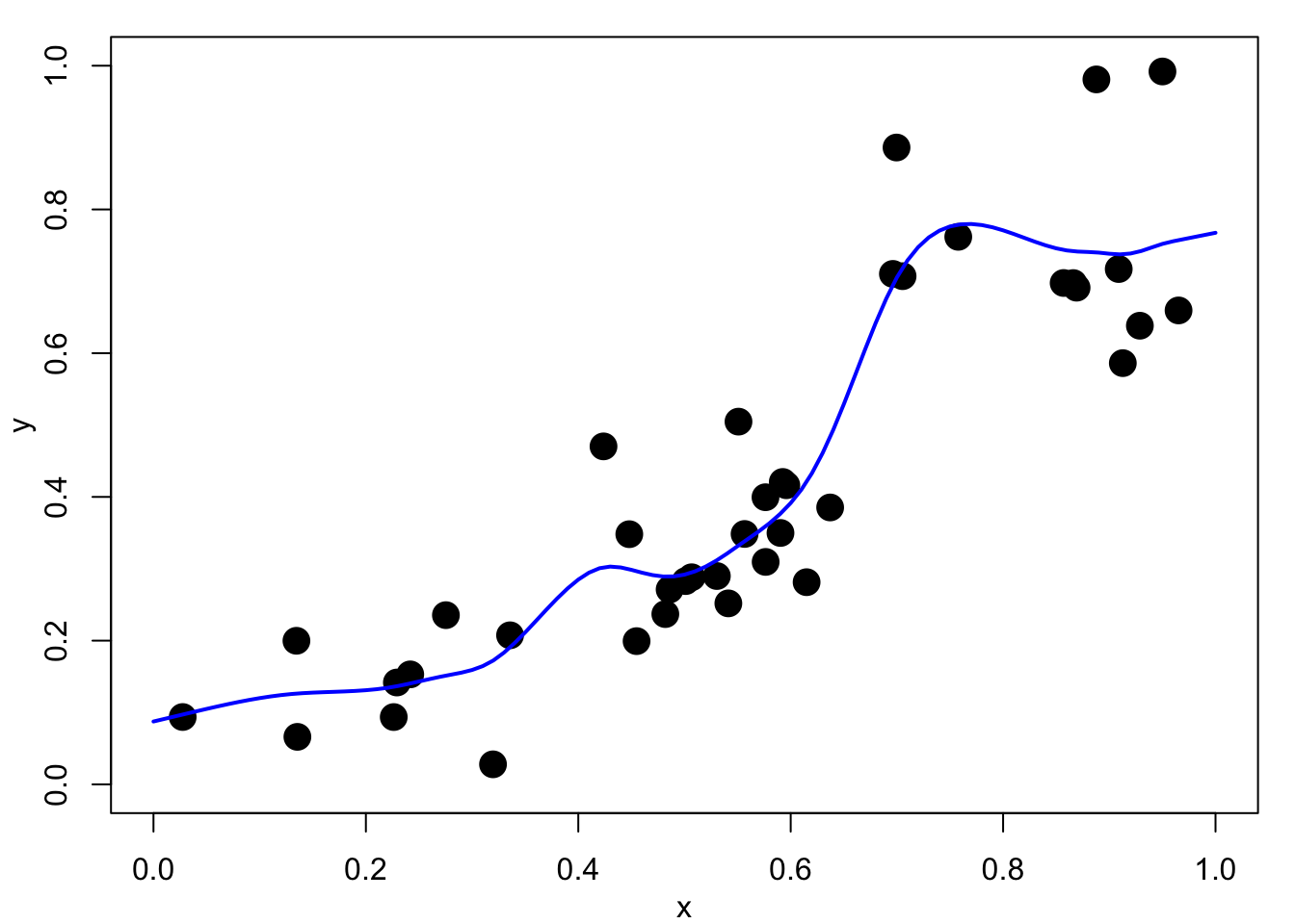
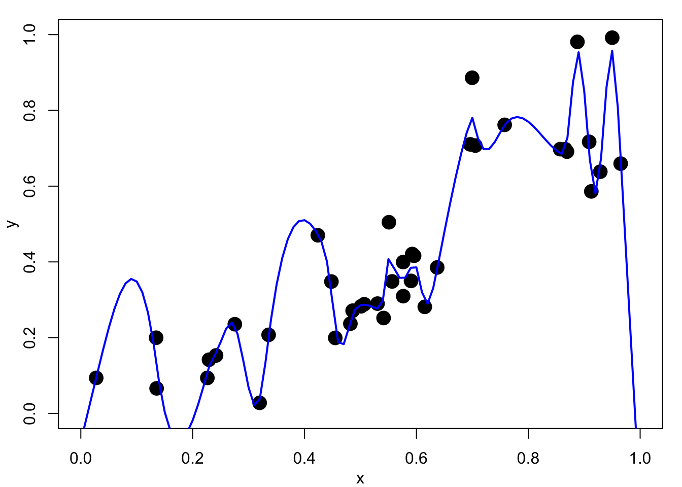
Figure 12.2 shows example smoothing spline fits using a range of smoothing parameters, \(\lambda\). In Figure 12.2 (a) the fit is essentially a straight line; perhaps Figure 12.2 (b) and Figure 12.2 (c) show acceptable fits. Figure 12.2 (d), with a very small \(\lambda\) value, is close to an interpolating spline fit and is clearly unacceptable.
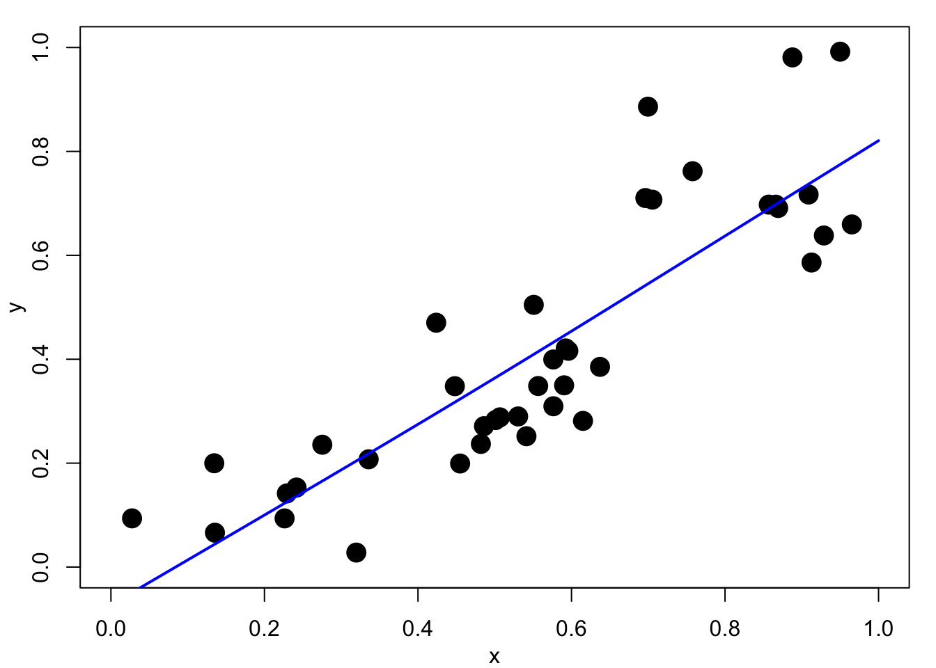
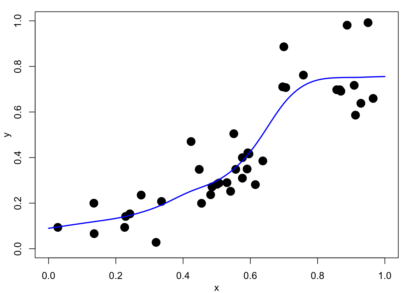
As the smoothing parameter \(\lambda\) increases, the optimal \(f\) becomes smoother. In particular, it can be shown that as \(\lambda \rightarrow \infty\), the vector of coefficients \({\mathbf b} \rightarrow {\mathbf 0}\), and \({\mathbf a}\) tends to the usual least-squares estimate of the regression parameters. Thus, the smoothing spline converges to the sample mean \(f(x)=\bar y\) when \(\nu=1\), and to the ordinary least squares fitted line, \(f(x)=\hat\alpha+\hat\beta x\), when \(\nu=2\). In the other direction, as \(\lambda \rightarrow 0\) the smoothing solution converges to the interpolating spline.
Test your knowledge recall and comprehension to reinforce basic ideas about smoothing splines.
Which of the following statements is NOT true?
Which of the following statements is true about splines?
Which of the following best describes the result of using a very large value of λ in a cubic smoothing spline?
Which of the following best describes the result of using a very small value of λ in a linear smoothing spline?
Which of the following statements best describes how to choose the value of λ?
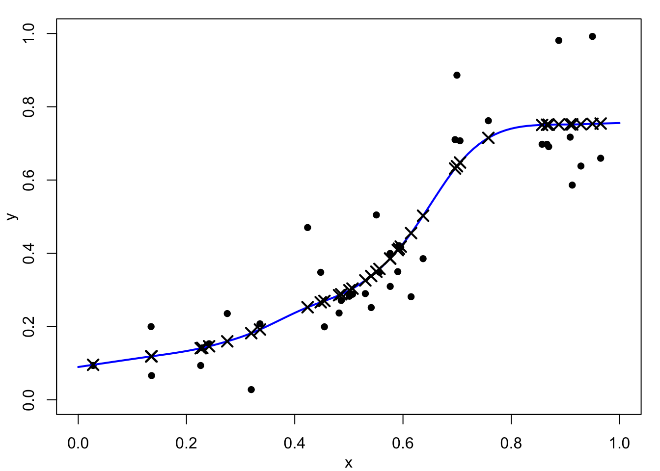
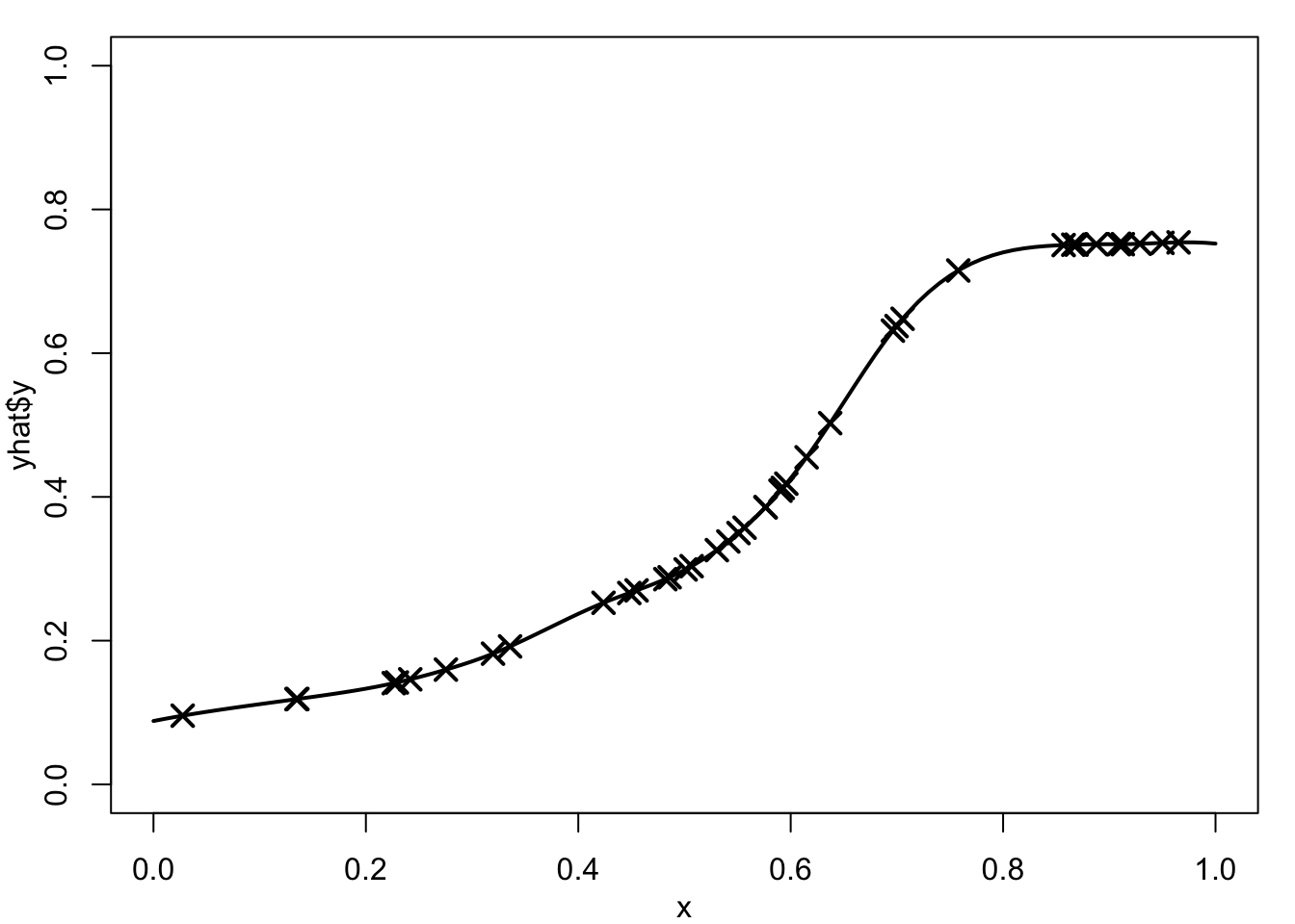
We show in the following proposition that the function \(f\) which minimizes Equation 12.2 is the interpolating spline of its fitted values.
Proposition 12.1 Suppose \(\hat{f}\) minimizes \(R_\nu(f,\lambda)\) and let \(\hat{y}_i = \hat{f}(x_i), i=1,\dots,n\) denote the corresponding fitted values. Then, \(\hat{f}\) solves the interpolation problem for the artificial data set \((x_i,\hat{y}_i), i=1,\dots , n\). That is, \(\hat{f}\) minimizes \(J_\nu(f)\) over functions \(f\) satisfying \(\hat f(x_i)=\hat{y}_i\), \(i=1,\ldots,n\). Consequently, \(\hat{f}\) is a \(p^{\text{th}}\)-order natural spline, where \(p=2\nu-1\). This means that, when solving the smoothing problem, we only need consider spline functions given by the representations in Proposition 11.1.
Proof: Suppose the assertion is not true. In this case, we must be able to find a function \({\hat{f}^\star}\), say, which also interpolates the artificial data \((x_i,\hat{y}_i), i=1,\dots ,n\), but which has a smaller roughness penalty. That is \[ J_\nu({\hat{f}^\star}) < J_\nu(\hat{f}) \mbox{ with } \hat{f}^\star(x_i) = \hat{y}_i, \ i=1,\ldots,n. \] Note that the fitted values from the function \(\hat f^\star\) are also equal to \(\hat y_i, i=1,\dots,n\) as it interpolates the same artificial data as \(\hat f\).
Now, from Equation 12.2, \[\begin{align*} R_\nu(\hat{f}^\star, \lambda) &= \sum_i (y_i-\hat{y}_i)^2 + \lambda J_\nu(\hat{f}^\star)\\ &< \sum_i (y_i-\hat{y}_i)^2 + \lambda J_\nu(\hat{f}) = R_\nu(\hat{f}, \lambda). \end{align*}\] Hence \(R_\nu(\hat{f}^\star, \lambda) < R_\nu(\hat{f}, \lambda)\). But, by construction \(\hat{f}\) minimizes \(R_\nu(f, \lambda),\) which is a contradiction. Hence, it must not be possible to find a function \({\hat{f}^\star}\) which also interpolates the artificial data but which has a smaller roughness penalty.
We have shown that \(\hat{f}\) is the optimal interpolant of the fitted values \(\hat{y}_i,\ i=1,\dots,n,\) so it follows from Proposition 11.1 that \(\hat{f}\) is a natural spline of order \(p=2\nu-1\).
We have just proved that the function \(\hat{f}\) that minimizes \(R_\nu (f, \lambda)\) must be a natural spline (linear if \(\nu=1\), cubic if \(\nu=2\)) with knots at \(\{x_i,\,i=1,\ldots,n\}.\) That is, as in Proposition 11.1, we can write:
\[ \hat{f}(t) = \sum_{i=1}^n b_i\left|t-x_i\right|^p + \begin{cases} a_0, &\nu=1\\ a_0 + a_1t, &\nu=2, \end{cases} \tag{12.3}\] where \(p=2\nu-1\) and constraints \[ \sum_{i=1}^n b_i = 0 \, \mbox{ for }\, \nu=1 \qquad \sum_{i=1}^n b_i = \sum_{i=1}^n b_i \, x_i = 0 \, \mbox{ for }\, \nu=2. \tag{12.4}\]
However, we have not yet figured out how to calculate the parameter values \(\hat{a}_0,\dots,\hat{a}_{\nu-1},\ \hat{b}_1,\dots,\hat{b}_n\) in Equation 12.3 which optimally fit the data \(y_1,\dots,y_n\). For this, it is convenient to re-express the penalised sum of squared residuals Equation 12.2 in matrix notation.
Proposition 12.2 The roughness of a natural linear spline \((\nu=1\), i.e. \(p=1)\) is \[ J_1(f) = -2\sum_{i=1}^n \sum_{k=1}^n b_i b_k \left| x_i - x_k \right| = c_1\,{\mathbf b}^T \, K_1 \, {\mathbf b}, \tag{12.5}\] and the roughness of a natural cubic spline (\(\nu=2\), i.e. \(p=3\)) is \[ J_2(f) = 12\sum_{i=1}^n \sum_{k=1}^n b_i b_k \left| x_i - x_k \right|^3 = c_2\,{\mathbf b}^T \, K_2 \, {\mathbf b}, \tag{12.6}\] where the constants are given by \[ c_1=-2, \quad c_2=12. \tag{12.7}\] Here \({\mathbf b}=(b_1,\ldots,b_n)^{T}\) is the vector of spline coefficients and \(K_\nu\) is the \(n\times n\) matrix whose \((i,k)\)th element is \(\left| x_i - x_k \right|^p\), where \(p=2\nu-1\), that is \[ K_\nu = \begin{bmatrix} |x_1-x_1|^p & |x_1-x_2|^p & \dots & |x_1-x_n|^p \\ |x_2-x_1|^p & |x_2-x_2|^p & \dots & |x_2-x_n|^p \\ \vdots & \vdots &\ddots & \vdots \\ |x_n-x_1|^p & |x_n-x_2|^p & \dots & |x_n-x_n|^p. \end{bmatrix} \]
Proof: See the supplementary notes proof_smoothing_spline_solution.pdf.
From Proposition 12.2 the roughness penalty satisfies: \[ J_\nu (\hat{f}) = c_\nu \, {\mathbf b}^T K_\nu {\mathbf b}, \tag{12.8}\] where \(c_1=-2\); \(c_2= 12\); \({\mathbf b}=(b_1,\ldots,b_n)^T\); and \(K_\nu\) is the \(n \times n\) matrix whose \((i,k)\)th element is \(\left|x_i-x_k\right|^p\).
From Equation 12.3, the value of \(\hat{f}\) at data location \(x_k\) is \[ \hat{f}(x_k) = \sum_{i=1}^n b_i\left|x_k-x_i\right|^p + \begin{cases}a_0, &\nu=1\\ a_0 + a_1x_k, &\nu=2 \end{cases}. \tag{12.9}\]
In matrix form, this is \[ \mathbf{\hat{f}} = \left[ \begin{array}{c}\hat{f}(x_1) \\ \vdots \\ \hat{f}(x_n)\end{array} \right] = K_\nu {\mathbf b} + L_\nu \mathbf{a}_{\,\nu} \tag{12.10}\] where \[ L_1 = \left[ \begin{array}{c} 1\\ \vdots \\ 1\end{array}\right], \quad \mathbf{a}_1 = a_0, \quad \quad \mbox{and} \quad \quad L_2 = \left[ \begin{array}{cc} 1 & x_1 \\ \vdots & \vdots \\ 1 & x_n \end{array} \right], \quad \mathbf{a}_2 = \left[\begin{array}{l}a_0\\a_1\end{array} \right] . \]
Thus, from Equation 12.4 – Equation 12.10, the penalised least-squares criterion Equation 12.2 reduces to a quadratic function of the parameters \(\mathbf{a}\) and \({\mathbf b}\):
\[ R_\nu(f, \lambda) = (\mathbf{y} - K_\nu \, {\mathbf b} - L_\nu \, \mathbf{a})^T (\mathbf{y} - K_\nu \, {\mathbf b} - L_\nu \, \mathbf{a}) + \lambda \,c_\nu \,{\mathbf b}^T K_\nu \,{\mathbf b} \tag{12.11}\] subject to \[ L_\nu^T\,{\mathbf b} = 0, \tag{12.12}\] where \(\mathbf{y} = (y_1,\ldots,y_n)^T\).
To find the explicit values for \(\mathbf{b}\) and \(\mathbf{a}\), we must minimize the quadratic function Equation 12.11 subject to the linear constraints Equation 12.12.
Proposition 12.3 The solution to the smoothing spline problem is given by \[ \begin{bmatrix} \hat{\mathbf a} \\ \hat{\mathbf b} \end{bmatrix} = \begin{bmatrix} 0 & L_\nu \\ L_\nu^T & K_\nu+\lambda^* I_n \end{bmatrix}^{-1} \begin{bmatrix} {\mathbf 0} \\ {\mathbf y} \end{bmatrix} \tag{12.13}\] and \(\lambda^* = c_\nu \lambda\).
Proof: See the supplementary notes proof_smoothing_spline_solution.pdf.
Fitting a smoothing spline to data involves estimating values of \(\mathbf a\) and \(\mathbf b\) to minimize the penalised roughness measure in Equation 12.11 subject to the constraints in Equation 12.12, which yields the explicit solution in Equation 12.13.
Of course, it is possible to code the solution of this matrix system, but it is usual instead to use in-built commands in software such as R.
In R the basic command is:
smooth.spline(x, y, lambda)where x and y are vectors of data coordinates, and lambda specifies the value of the smoothing parameter to use – note that the effect of a given value of \(\lambda\) depends on the problem considered.
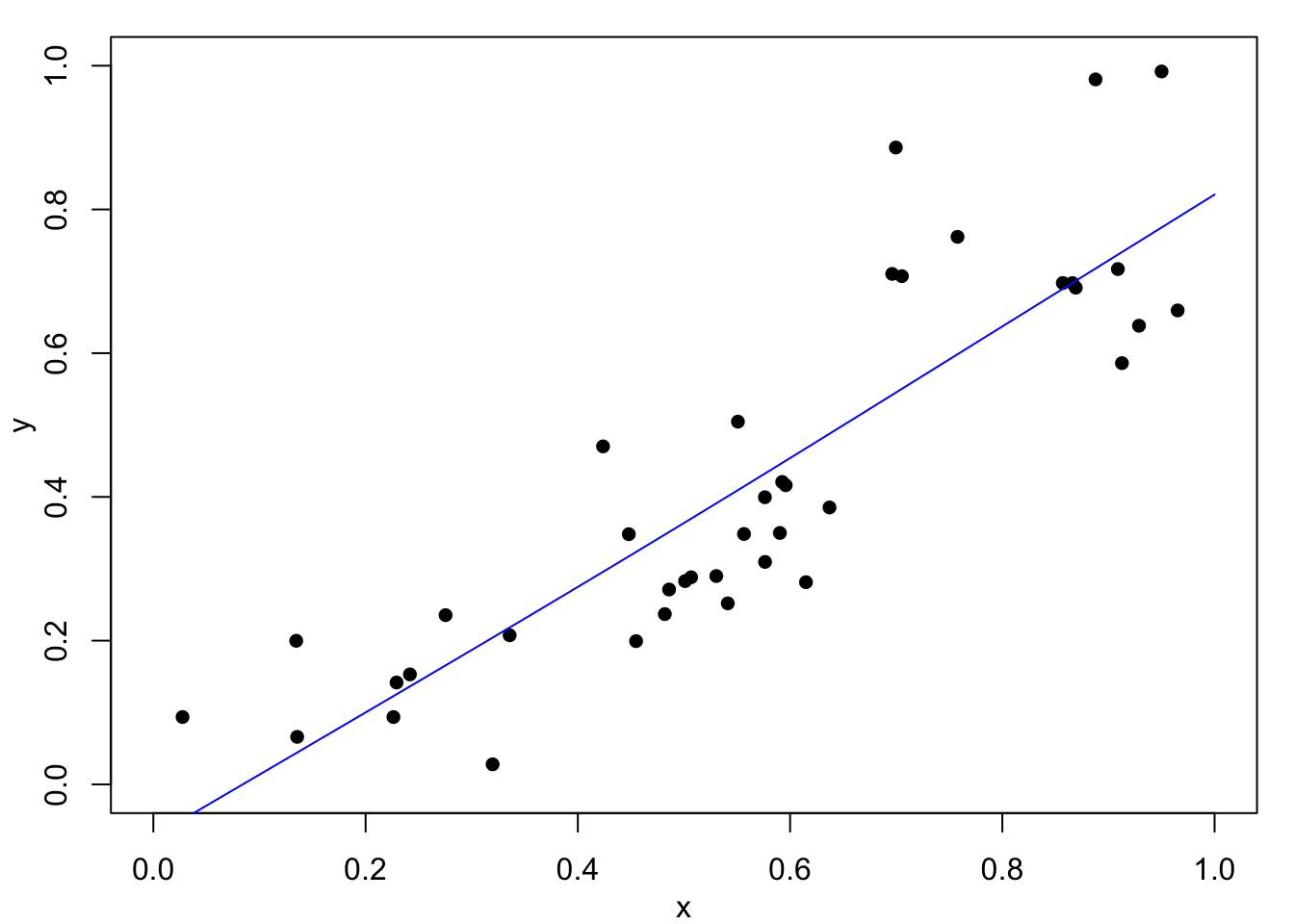
For example, consider the synthetic data set containing a break-point at \(x=2/3\) first seen in Figure 9.2. Fitted spline curves with \(\lambda=0.00001\) and \(\lambda=1\), shown in Figure 12.4, are based on the following commands:
myfit1 = smooth.spline(x, y, lambda = 0.00001)
myfit2 = smooth.spline(x, y, lambda = 1)par(mar=c(3,3,1,1), mgp=c(2,1,0))
set.seed(12341)
x = runif(40)
y = 0.75*(x >= 0.67) + 0.6*x*(x<0.67) + rnorm(40,0,0.1)
plot(x,y, xlim=c(0,1), ylim=c(0,1), pch=16)
myfit1 = smooth.spline(x, y, lambda = 0.00001)
fit.locations = seq(0,1,0.01)
fitted = predict(myfit1, fit.locations)
lines(fitted, col="blue")
plot(x,y, xlim=c(0,1), ylim=c(0,1), pch=16)
myfit2 = smooth.spline(x, y, lambda = 1)
fit.locations = seq(0,1,0.01)
fitted = predict(myfit2, fit.locations)
lines(fitted, col="blue")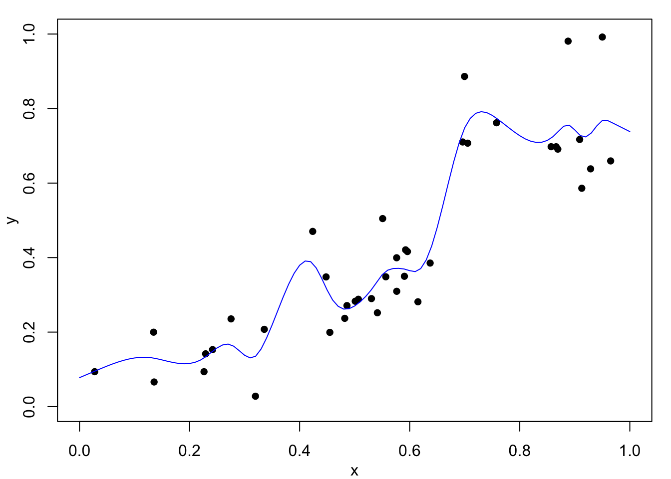
If no value of the smoothing parameter is specified, the optimal value is calculated using generalised cross-validation as discussed in the next chapter.
12.1 The following data record the number of tropical cyclones in each of 13 seasons (Dobson and Barnett, 3rd edn, Table 1.2):
| Season | 1 | 2 | 3 | 4 | 5 | 6 | 7 | 8 | 9 | 10 | 11 | 12 | 13 |
| No of cyclones | 6 | 5 | 4 | 6 | 6 | 3 | 12 | 7 | 4 | 2 | 6 | 7 | 4 |
Follow the R code used in Section 12.5 but don’t worry about finding an exact value for the smoothing parameter, only the order of magnitude.
12.2 Consider the Old Faithful data set on geyser eruptions available in R. Use the following commands to learn more about and visualize the data:
data(faithful)
help(faithful)
plot(faithful)
Fit a cubic smoothing spline to these data, using a range of values for the smoothing parameter \(\lambda\). By eye, suggest a suitable value for \(\lambda\).
Taking waiting as the explanatory variable and eruptions as the response, follow the R code used in Section 12.5 but don’t worry about finding an exact value for the smoothing parameter, only the order of magnitude.