A parametric survival model specifies a functional form for \(S(t)\) (or equivalently \(h(t)\)) up to a finite number of unknown parameters. The parameters are then estimated from data by maximum likelihood. This chapter introduces the most important parametric families.
Key properties: - Constant hazard: the risk of dying does not increase or decrease with time (memoryless property). - Mean: \(\E[T] = 1/\lambda\); Median: \(\mu_{1/2} = \log 2/\lambda\). - Simple to fit and interpret, but often too restrictive in practice.
The shape parameter \(\gamma\) controls how the hazard changes with time:
\(\gamma\)
Hazard
Interpretation
\(< 1\)
Decreasing
Early high risk, then improving (“infant mortality”)
\(= 1\)
Constant
Exponential model
\(> 1\)
Increasing
Ageing / wear-out
The Weibull distribution is the most widely used parametric model in survival analysis because of its flexibility and its proportional hazards property (see Chapter 21).
18.4 Other parametric families
Gompertz distribution:\[
h(t) = \lambda e^{\theta t}, \quad \lambda > 0, \;\theta \in \mathbb{R}.
\] The hazard grows exponentially with \(t\). Used extensively in actuarial science to model human mortality.
Gamma distribution with shape \(\alpha > 0\) and rate \(\lambda > 0\): \[
f(t) = \frac{\lambda^\alpha t^{\alpha-1}}{\Gamma(\alpha)} e^{-\lambda t}.
\] The hazard starts at 0 if \(\alpha > 1\), at \(\infty\) if \(\alpha < 1\), and at \(\lambda\) if \(\alpha = 1\) (exponential). Unlike the Weibull, the gamma does not have the proportional hazards property.
Log-normal distribution: \(\log T \sim \mathrm{N}(\mu, \sigma^2)\). The hazard first increases then decreases (hump-shaped). Common in engineering reliability.
18.5 Graphical assessment of parametric fit
Before fitting a model, it is useful to inspect the data graphically to see which family is plausible.
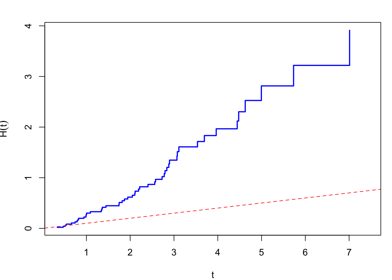
Exponential check. The Kaplan–Meier estimate of \(H(t) =
-\log\widehat{S}(t)\) should be approximately linear through the origin: \[
H(t) = \lambda t \quad \Rightarrow \quad \widehat{H}(t) \approx \lambda t.
\]
Weibull check. Taking logs of \(H(t) = \lambda t^\gamma\): \[
\log H(t) = \log\lambda + \gamma\log t.
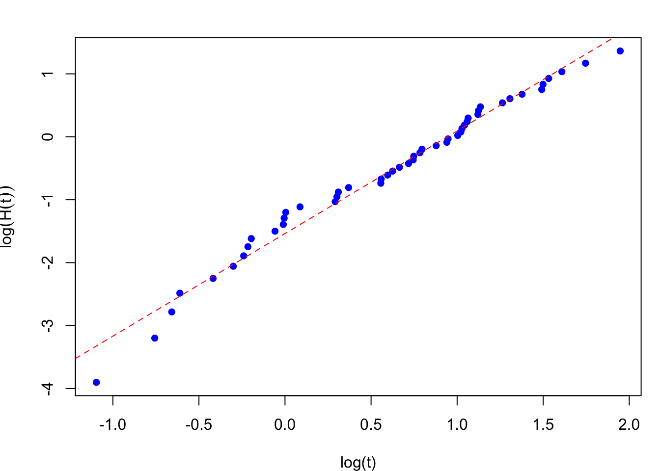
\] A plot of \(\log\widehat{H}(t)\) against \(\log t\) (the log-cumulative hazard plot) should be approximately linear. The slope estimates \(\gamma\) and the intercept estimates \(\log\lambda\).
(a) Cumulative hazard vs time
(b) Log-cumulative hazard vs log time
Figure 18.1: Log-cumulative hazard plots for simulated Weibull data. The left panel shows \(\widehat{H}(t)\) vs \(t\) (exponential check); the right panel shows \(\log\widehat{H}(t)\) vs \(\log t\) (Weibull check). The linear trend on the right confirms the Weibull fit.
18.6 Simulation and fitting in R
Code
library(survival)# Simulate Weibull data with shape gamma=2, scale lambda=0.1set.seed(42)gamma <-2; lambda <-0.1t_sim <-rweibull(100, shape = gamma, scale = lambda^(-1/gamma))# Fit Weibull model (no censoring)fit <-survreg(Surv(t_sim) ~1, dist ="weibull")summary(fit)# Convert R's AFT parametrisation to PH parametrisation:# R uses log(T) = mu + sigma * W where W ~ Gumbel# gamma_hat = 1 / fit$scale# lambda_hat = exp(-gamma_hat * coef(fit))gamma_hat <-1/ fit$scalelambda_hat <-exp(-gamma_hat *coef(fit))cat("gamma:", gamma_hat, "\n")cat("lambda:", lambda_hat, "\n")
Note: R’s parametrisation
The survreg() function uses an accelerated failure time (AFT) parametrisation. For a Weibull model, the output reports an intercept \(\mu\) and a scale \(\sigma\). To convert to the hazard parametrisation \(h(t) = \lambda\gamma t^{\gamma-1}\): \[
\hat\gamma = 1/\hat\sigma, \qquad \hat\lambda = e^{-\hat\gamma\hat\mu}.
\]
Exercises
18.1. Two groups of patients have the following survival times (in days), with right-censored times marked \(^*\):
For each group, estimate the percentiles \(t(P)\) for \(P = 10, 20, \ldots, 90\) from the KM table. Arrange your results in a two-column table.
The \(P\)th percentile satisfies \(S(t(P)) = 1 - P/100\). Because \(\hat{S}(t)\) is a step function (not a smooth curve), do not interpolate: \(t(P)\) is simply the smallest observed event time at which \(\hat{S}(t)\) first drops to or below \(1-P/100\).
For each group, produce the graphical Weibull check: plot \(\log\widehat{H}(t)\) against \(\log t\), where \(\widehat{H}(t) = -\log\widehat{S}(t)\), using the KM jump points from the tables above. Do the plots support a Weibull model for each group’s survival times?
From your plots in (b), read off rough graphical estimates of the shape \(\gamma\) and (via the intercept) the scale \(\lambda\) for each group.
Recall \(\widehat{H}(t) = -\log\widehat{S}(t)\), and under a Weibull model \(\log H(t) = \log\lambda + \gamma\log t\), so plot \(\log\widehat{H}(t)\) against \(\log t\): the slope of the best-fit line estimates \(\gamma\), and the intercept estimates \(\log\lambda\).
18.2. Using the raw survival data (times and censoring indicators) from Exercise 18.1, fit a Weibull model separately to each group in R.
Write the R code to fit each model and report \(\hat\gamma\) and \(\hat\lambda\) for each group, using the parametrisation conversion given earlier in this chapter. How do these compare with your graphical estimates from 18.1(c)?
The two groups have similar estimated shape parameters \(\hat\gamma\). Since the hazards are \(h(t) = \lambda\gamma t^{\gamma - 1}\), when \(\gamma\) is (approximately) the same for both groups the ratio of hazards is approximately \(\hat\lambda_{\text{I}}/\hat\lambda_{\text{II}}\). Compute this ratio and interpret it: which group has the worse survival experience, and by roughly what factor?
Use survreg(Surv(t, d) ~ 1, dist = "weibull") separately on each group’s data, with d = 1 for an event and d = 0 for a censored time (matching the \(^*\) superscripts in Exercise 18.1). Convert to the hazard parametrisation via \(\hat\gamma = 1/\hat\sigma\), \(\hat\lambda = e^{-\hat\gamma\hat\mu}\), as in the “R’s parametrisation” note above.