17 Kaplan–Meier Estimator
17.1 Overview
When data include censored observations, the empirical survival function of Chapter 16 is biased. The Kaplan–Meier (KM) estimator is the non-parametric maximum likelihood estimator of \(S(t)\) that correctly accounts for right censoring. It is the standard starting point for any survival analysis.
17.2 The product-limit formula
Let \(t_{(1)} < t_{(2)} < \cdots < t_{(k)}\) denote the ordered, distinct event times (ignoring censored observations). For each event time \(t_{(j)}\), define:
- \(n_j\) = number of individuals at risk (alive and uncensored) immediately before \(t_{(j)}\),
- \(d_j\) = number of events (deaths) at \(t_{(j)}\).
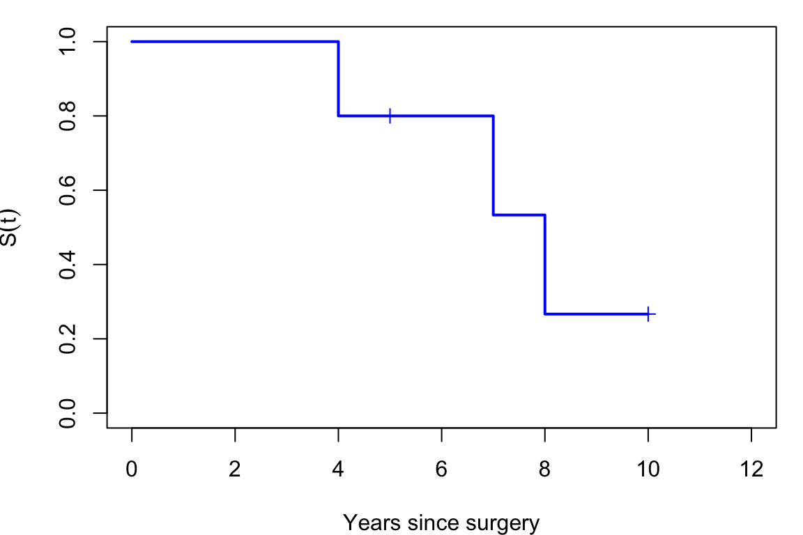
This is a step function that drops at each observed event time. Between event times, \(\widehat{S}(t)\) is constant. Censored observations contribute to the risk set \(n_j\) before they are censored but do not cause the estimator to drop.
17.3 Standard error: Greenwood’s formula
Since the KM estimator is random, we need a measure of its precision. Greenwood’s formula gives the approximate variance:
\[ \widehat{\text{Var}}\bigl(\widehat{S}(t)\bigr) = \widehat{S}(t)^2 \sum_{j:\, t_{(j)} \leq t} \frac{d_j}{n_j(n_j - d_j)}. \]
An approximate \(95\%\) pointwise confidence interval for \(S(t)\) is
\[ \widehat{S}(t) \pm 1.96 \sqrt{\widehat{\text{Var}}\bigl(\widehat{S}(t)\bigr)}. \]
In practice, confidence intervals based on the log-log transformation of \(S(t)\) are preferred because they automatically respect the constraint \(0 < S(t) < 1\) (the plain linear interval can exceed these bounds). These are computed automatically by survfit() in R.
17.4 The delta method
Constructing a confidence interval on a transformed scale, as above, requires the variance of the transformed quantity, not just of \(\widehat{S}(t)\) itself. The delta method provides a general way to approximate the variance of a function of an estimator, given the variance of the estimator itself.
This is exactly how the log-log and logit transformations of \(\widehat{S}(t)\) are handled: apply the delta method with \(g\) equal to the chosen transformation, substitute Greenwood’s formula for \(\mathrm{Var}(\widehat{S}(t))\), construct the interval on the transformed scale, and back-transform via \(g^{-1}\) to recover a confidence interval for \(S(t)\) that automatically respects \(0 < S(t) < 1\).
17.5 Kaplan–Meier in R
Code
library(survival)

t     <- c(4, 5, 7, 8, 10)
delta <- c(1, 0, 1, 1, 0)

# Fit KM estimator
km <- survfit(Surv(t, delta) ~ 1)
summary(km)

# Plot with confidence band
plot(km, conf.int = TRUE, mark.time = TRUE, col = "blue", lwd = 2,
     xlab = "Time", ylab = "S(t)")

# Estimated median
km  # median and 95% CI printed in default output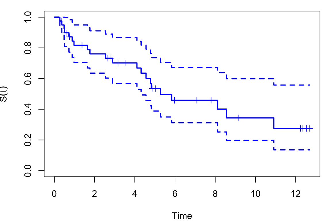
17.6 Two-group comparison
When we have two groups (e.g., treatment vs control), we can compare their KM curves visually and test for equality using the log-rank test. In R:
Code
# Two groups: group = 0 (control), group = 1 (treatment)
km_grouped <- survfit(Surv(t, delta) ~ group)
plot(km_grouped, col = c("blue", "red"), lwd = 2,
     xlab = "Time", ylab = "S(t)",
     legend.text = c("Control", "Treatment"))

# Log-rank test
survdiff(Surv(t, delta) ~ group)Exercises
17.1. The following are survival times (in months) for ten colorectal cancer patients: \[2,\ 10,\ 14,\ 27,\ 27,\ 37,\ 44,\ 46,\ 54,\ 60.\] All ten times are exact (no censoring in this part).
Compute the empirical survival function \(\hat{S}(t)\) and sketch it. Estimate the median survival time from the plot.
Now suppose the observation at \(t = 44\) months is instead a right-censored time (the patient was still alive at 44 months). Re-compute the survival estimate using the Kaplan–Meier method, showing all working. State how the estimates \(\hat{S}(46)\) and \(\hat{S}(54)\) change compared with part (a).
For the KM estimator, at each event time \(t_{(j)}\) with \(d_j\) events and risk set \(n_j\): multiply the running product by \((n_j - d_j)/n_j\). Censored observations reduce the risk set at the next event time but do not contribute a multiplicative factor of their own.
For part (a), use library(survival) and survfit(Surv(t, d) ~ 1). For part (b), Greenwood’s formula is \(\widehat{\mathrm{Var}}(\hat{S}(t)) = [\hat{S}(t)]^2 \sum_{t_{(j)} \leq t} d_j / (n_j(n_j - d_j))\).
Reproduce the KM analysis from Exercise 17.1(b) in R. Plot the KM curve with 95% confidence bands.
Using Greenwood’s formula, compute an approximate 95% confidence interval for \(S(11)\) (the probability of surviving beyond 11 months). Work by hand.
17.3. Let \(\hat{S}(t)\) be the Kaplan–Meier estimator and define the logit transform \[\hat{S}_{\text{logit}}(t) = \log\!\left(\frac{\hat{S}(t)}{1-\hat{S}(t)}\right).\]
Using the delta method and Greenwood’s formula, derive an expression for the approximate variance of \(\hat{S}_{\text{logit}}(t)\).
Explain how this variance can be used to construct a confidence interval for \(S(t)\) that is guaranteed to lie in \((0,1)\).
Let \(g(x) = \log(x/(1-x))\). Compute \(g'(x)\) and apply the delta method: \(\mathrm{Var}(g(\hat{S}(t))) \approx [g'(S(t))]^2\,\mathrm{Var}(\hat{S}(t))\). Then substitute Greenwood’s formula. For part (b), construct the CI on the logit scale and back-transform via the inverse logit.