We have now covered all the core elements of generalised linear models. This chapter consolidates those ideas by revisiting the three-component structure of a GLM, summarising the key results from earlier chapters, and working through a complete analysis from start to finish. We then look forward to Part II, where we will relax the linearity assumption on the systematic component.
8.2 The three-component structure revisited
Every generalised linear model has exactly three components:
Random component. The response variable \(Y_i\) follows a distribution from the exponential family: \[f(y_i;\theta_i,\phi) = \exp\left\{\frac{y_i\theta_i - b(\theta_i)}{\phi} + c(y_i,\phi)\right\}.\] The mean and variance are determined by \(b(\theta_i)\): \[\mathrm{E}[Y_i] = b'(\theta_i) = \mu_i, \qquad
\mathrm{Var}[Y_i] = \phi\, b''(\theta_i).\]
Systematic component. A linear predictor in the explanatory variables: \[\eta_i = \mathbf{x}_i^T\boldsymbol{\beta} = \sum_{j=1}^p \beta_j x_{ij}.\]
Link function. A monotone differentiable function \(g\) connecting mean to linear predictor: \[g(\mu_i) = \eta_i.\] When \(g = (b')^{-1}\), the link is canonical and simplifies the score equations.
The following table summarises the choices for the three distributions we have studied in detail.
Table 8.1: Summary of GLM components for the three standard exponential family distributions.
Distribution
Canonical link
Variance function
Typical use
Normal
Identity: \(\eta = \mu\)
\(b''(\theta)=1\)
Continuous response
Binomial
Logit: \(\eta = \log\frac{p}{1-p}\)
\(b''(\theta)=mp(1-p)\)
Counts / proportions
Poisson
Log: \(\eta = \log\lambda\)
\(b''(\theta)=\lambda\)
Count data
8.3 Fitting, inference, and model comparison
Estimation. Parameters are estimated by maximum likelihood using the iteratively reweighted least squares (IRLS) algorithm (see the supplementary notes proof_IRLS.pdf for the full derivation). The MLE satisfies asymptotically: \[\hat{\boldsymbol\beta} \sim N_p\!\left(\boldsymbol\beta,\, \mathcal{J}^{-1}(\boldsymbol\beta)\right).\]
Deviance. The deviance measures how much a fitted model \(M\) falls short of the saturated model: \[D = 2\phi\left\{l(\tilde{\boldsymbol\theta};\mathbf{y},\phi) -
l(\hat{\boldsymbol\theta};\mathbf{y},\phi)\right\}.\] For the three standard families, \(D\) reduces to:
Normal: residual sum of squares \(\sum_i(y_i-\hat\mu_i)^2\).
Model comparison. For two nested models \(M_1 \subset M_2\) with \(r_1 < r_2\) parameters:
If \(\phi\) is known: \((D_1-D_2) \sim \chi^2_{r_2-r_1}\) asymptotically.
If \(\phi\) is unknown: use the \(F\)-statistic Equation 4.19.
Residuals. Deviance residuals \(e_i^\text{dev} = \text{sign}(y_i-\hat\mu_i)\sqrt{d_i}\) and Pearson residuals \(e_i^P = (y_i-\hat\mu_i)/\sqrt{b''(\hat\theta_i)}\) are the main diagnostic tools.
8.4 Worked case study: Coronary heart disease
This example illustrates the complete GLM workflow: data exploration, model formulation, fitting, inference, and model criticism.
The data (Dobson and Barnett, 2008, p.127) relate to a study of coronary heart disease (CHD). A total of 1,329 men were cross-classified by cholesterol level (4 ordered groups: 1 = lowest, 4 = highest) and blood pressure (4 ordered groups: 1 = lowest, 4 = highest). For each of the \(4 \times 4 = 16\) cells, the number of men with CHD (\(y_{ij}\)) and the total number of men (\(m_{ij}\)) are recorded. The data are in https://www.richardpmann.com/MATH3701/Datasets/chd.txt.
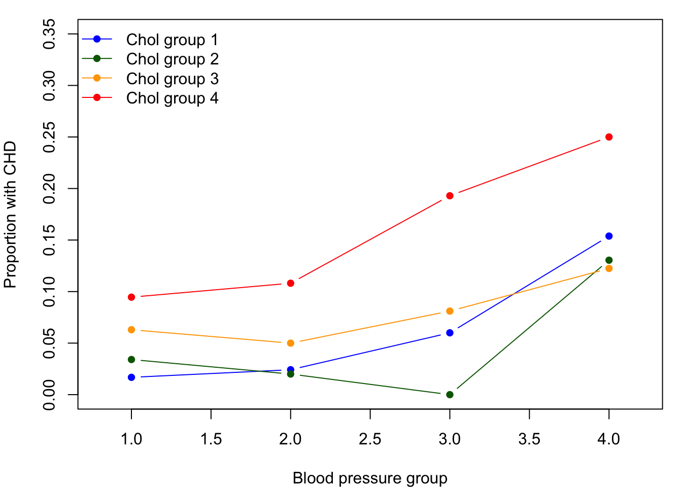
Figure 8.1: Proportion with CHD by cholesterol and blood pressure group. Lines connect groups at the same cholesterol level.
Both increasing cholesterol and increasing blood pressure appear associated with higher CHD proportions.
8.4.2 Step 2: Model formulation
Each \(Y_{ij}\) is a count of CHD cases out of \(m_{ij}\) men, so a Binomial GLM with logit link is appropriate: \[Y_{ij} \sim \text{B}(m_{ij}, p_{ij}), \qquad
\text{logit}(p_{ij}) = \mu + \alpha_i + \beta_j,\] where \(\alpha_i\) is the effect of cholesterol group \(i\) and \(\beta_j\) is the effect of blood pressure group \(j\). We will also consider a saturated model (with an interaction term) and the null model.
Since both factors are ordered, we will first treat them as factors (to allow flexible effect estimates) and then consider whether a simpler model with numeric scores is adequate.
8.4.3 Step 3: Fit and compare models
Code
chd$cholF =as.factor(chd$chol)chd$bpF =as.factor(chd$bp)# Response matrix: successes and failuresym =cbind(chd$y, chd$m - chd$y)# Null modelglm0 =glm(ym ~1, family=binomial, data=chd)# Main effects model (independence)glm1 =glm(ym ~ cholF + bpF, family=binomial, data=chd)# Saturated model (with interaction)glm2 =glm(ym ~ cholF * bpF, family=binomial, data=chd)# Summary of deviancescat("Null deviance: ", round(glm0$deviance, 2),"on", glm0$df.residual, "df\n")
The main-effects model fits the data well (\(p > 0.05\)).
8.4.5 Step 5: Interpret the fitted model
Code
summary(glm1)
Call:
glm(formula = ym ~ cholF + bpF, family = binomial, data = chd)

Coefficients:
            Estimate Std. Error z value Pr(>|z|)
(Intercept) -3.48194    0.34865  -9.987  < 2e-16 ***
cholF2      -0.20798    0.46641  -0.446  0.65566
cholF3       0.56223    0.35080   1.603  0.10900
cholF4       1.34412    0.34297   3.919 8.89e-05 ***
bpF2        -0.04146    0.30365  -0.137  0.89139
bpF3         0.53236    0.33240   1.602  0.10925
bpF4         1.20042    0.32689   3.672  0.00024 ***
---
Signif. codes:  0 '***' 0.001 '**' 0.01 '*' 0.05 '.' 0.1 ' ' 1

(Dispersion parameter for binomial family taken to be 1)

    Null deviance: 58.7262  on 15  degrees of freedom
Residual deviance:  8.0762  on  9  degrees of freedom
AIC: 73.18

Number of Fisher Scoring iterations: 4
The estimated log-odds ratios for cholesterol and blood pressure groups (relative to group 1 in each case) show a clear increasing trend: higher cholesterol and higher blood pressure each increase the log-odds of CHD.
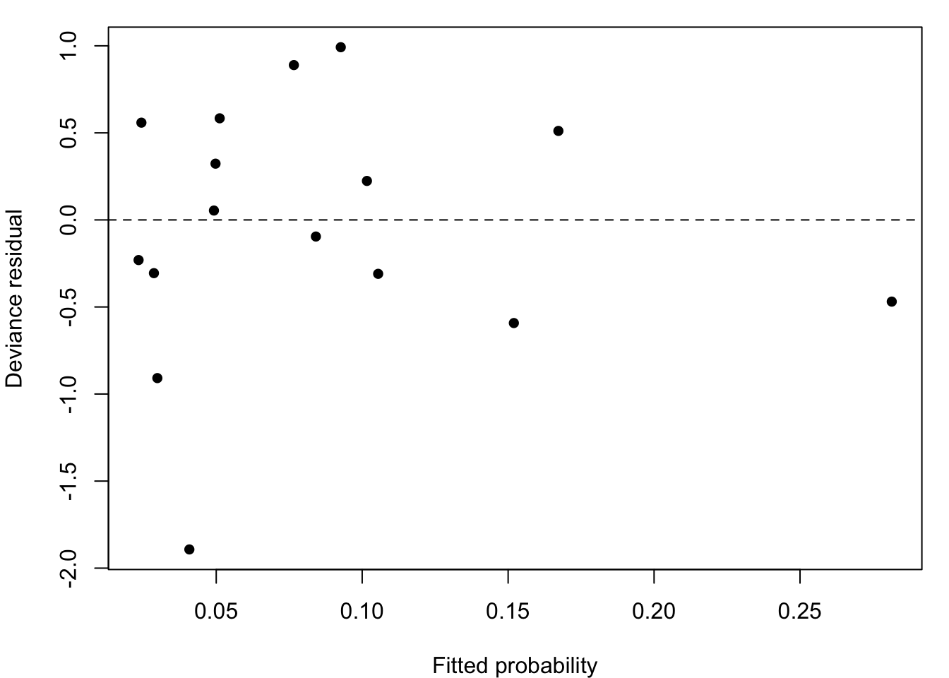
Figure 8.2: Deviance residuals from the main-effects logistic regression model.
No strong pattern is apparent, consistent with a well-fitting model.
8.5 Looking ahead: limitations of the linear predictor
The GLM framework is powerful, but the linearity constraint \(\eta_i = \mathbf{x}_i^T\boldsymbol{\beta}\) can be restrictive.
Consider a situation where the true relationship between a continuous explanatory variable \(x\) and the response is smooth but nonlinear. We have two broad options:
Polynomial regression: add \(x^2, x^3, \dots\) to the linear predictor. This is easy but can produce unstable fits and the polynomial degree must be chosen in advance.
Non-parametric smoothing: replace \(\beta x\) with a smooth function \(f(x)\) estimated from the data. This forms the basis of Generalised Additive Models (GAMs), studied in Part II.
The GAM model is written: \[g(\mu_i) = \alpha + f_1(x_{i1}) + f_2(x_{i2}) + \cdots + f_p(x_{ip}),\] where each \(f_j\) is a smooth function (a spline) chosen to fit the data while penalising excessive wiggliness.
We will see that GAMs retain the interpretability of GLMs while gaining considerable flexibility, and that the estimation and inference methods are natural generalisations of what we have developed in Part I.
8.6 Summary
Tip
Key points from Part I
A GLM is defined by its random component (exponential family), systematic component (linear predictor), and link function.
Maximum likelihood estimation is carried out by IRLS.
Model fit is assessed via deviance; nested models are compared by likelihood ratio tests (\(\chi^2\) or \(F\)).
Logistic regression (binomial/logit) is used for binary or proportion responses.
Log-linear models (Poisson/log) model count data; product-multinomial models arise when marginal totals are fixed.
Overdispersion (variance exceeding the theoretical value) can be addressed via quasi-likelihood.