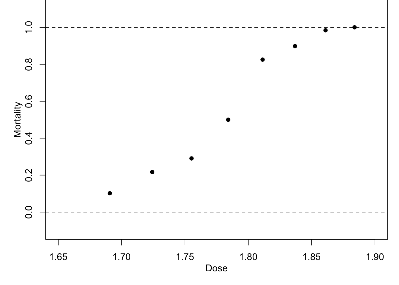
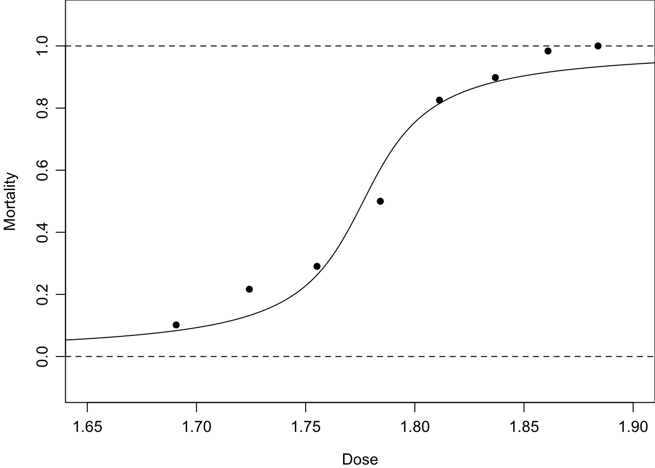
We cannot always assume that the dependent variable \(Y\) is normally distributed. For example, for the beetle mortality data in Table 1.1, suppose each beetle subjected to a dose \(x_i\) has a probability \(p_i\) of being killed. Then, the number of beetles killed \(Y_i\) out of a total number \(m_i\) at dose-level \(x_i\) will have a \(\text{Bin}(m_i,p_i)\) distribution with probability mass function
\[
\text{Pr}(y_i ;~ p_i,m_i) = \left(\begin{array}{c} m_i\\ y_i \end{array} \right) p_i^{y_i} (1-p_i)^{m_i-y_i}
\tag{3.1}\] where \(y_i\) takes values in \(\{0,1,\dots,m_i\}\).
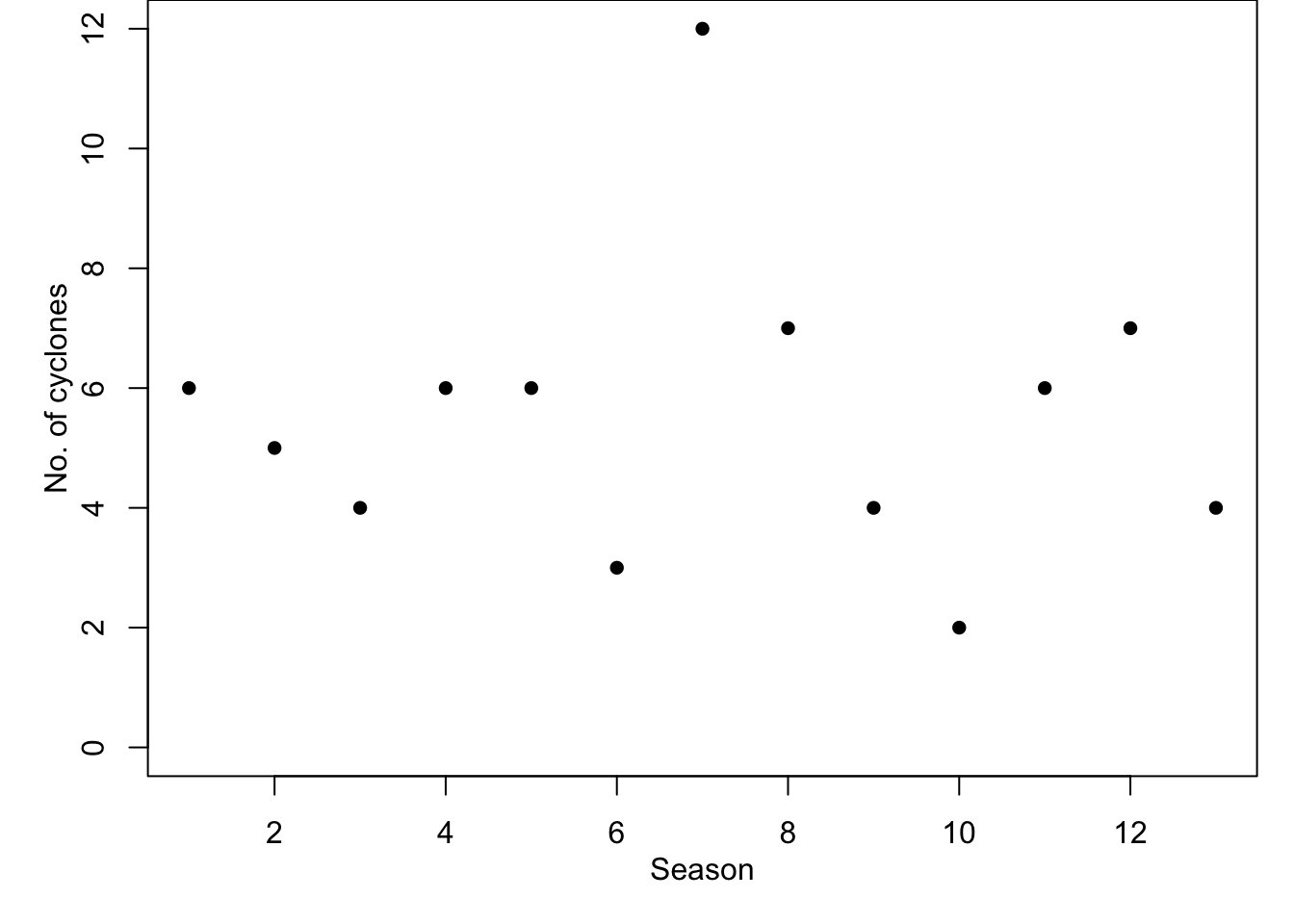
Table 12.1 contains seasonal data on tropical cyclones for 13 seasons. Suppose that, within season \(i\), there is a constant probability \(\lambda_i dt\) of a cyclone occurring in any short time-interval \(dt\). Then the total number of cyclones \(Y_i\) during season \(i\) will have a Poisson distribution with mean \(\lambda_i\), that is \(Y_i\sim \text{Po}(\lambda_i)\), with probability mass function \[
\text{Pr}(y_i ;~ \lambda_i) = \frac{\lambda_i^{y_i} e^{-\lambda_i} }{y_i!}
\tag{3.2}\] where \(y_i\) takes values in \(\{0,1,2,\dots\}\).
Table 3.1: Numbers of tropical cyclones in \(n = 13\) successive seasons1
Season
1
2
3
4
5
6
7
8
9
10
11
12
13
No of cyclones
6
5
4
6
6
3
12
7
4
2
6
7
4
In these two examples, we have non-normal data and would like to know whether and how the dependent variable \(Y_i\) depends on the explanatory variable dose or season.
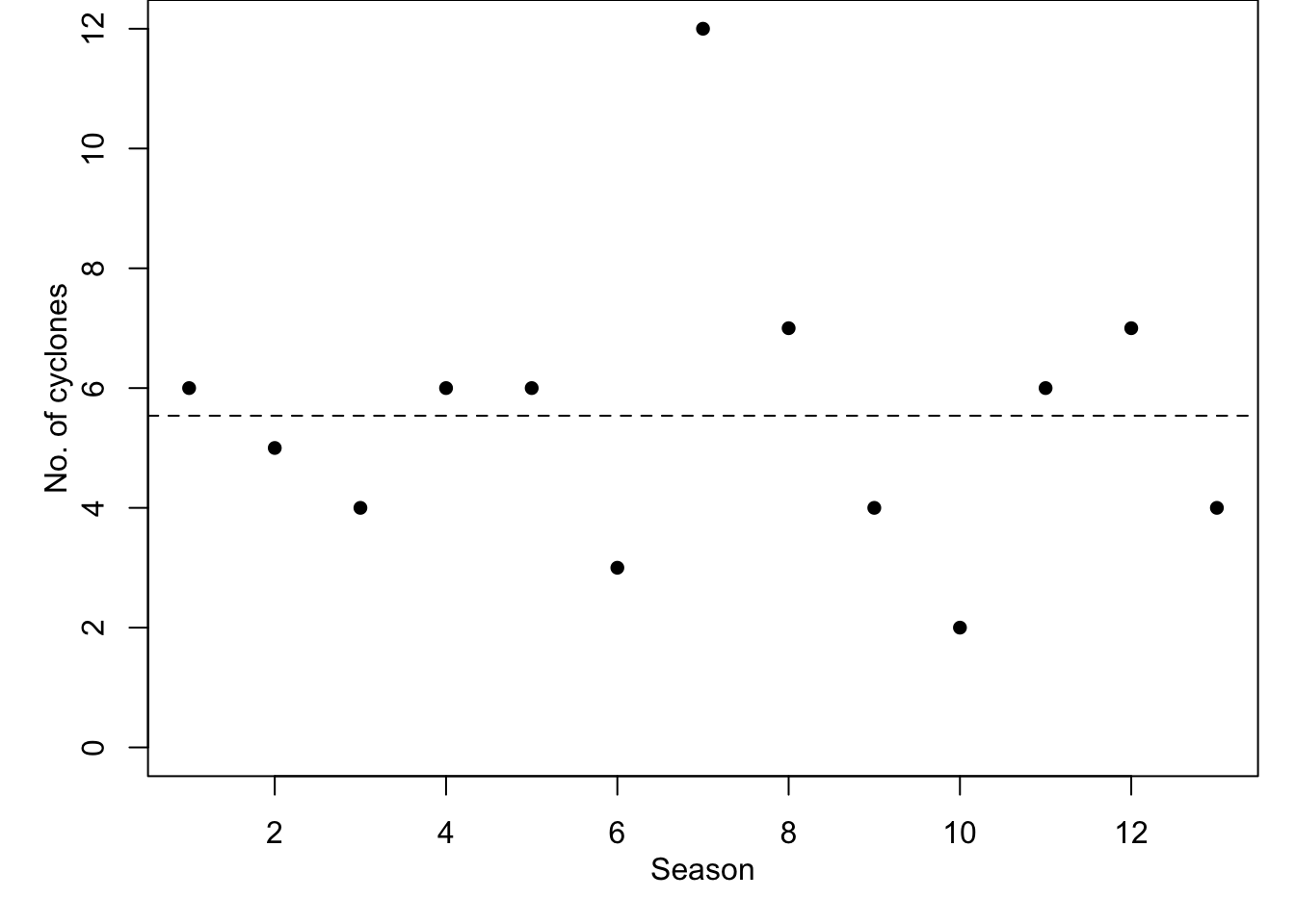
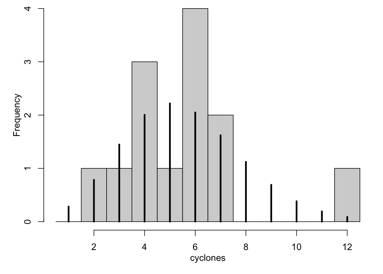
Figure 3.1: Examples of non-normally distributed data.
Generalised linear models provide a modelling framework for data analysis in the non-normal setting. We will revisit the beetle mortality and cyclone data sets after describing the structure of a generalised linear model.
Focus on distributions quiz
Test your knowledge recall and application to reinforce basic ideas and prepare for similar concepts later in the Chapter.
Which of the following best describes the sample space of a binomial random variable?
Which of the following best describes the sample space of a Poisson random variable?
Which of the following best describes the sample space of a normal random variable?
For the binomial distribution, which of the following best describes the range of values possible for log(p/(1-p))?
For the Poisson distribution, which of the following best describes the range of values possible for log(λ)?
For the normal distribution, which of the following best describes the range of values possible for µ?
3.2 The GLM structure
A generalised linear model relates a continuous or discrete response variable \(Y\) to a set of explanatory variables \(\mathbf{x}=(x_1, \ldots, x_p)\). The model contains three parts:
Random part: The probability (mass or density) function of \(Y\) is assumed to belong to the two-parameterexponential family of distributions with parameters \(\theta\) and \(\phi:\)
\[
f(y; \theta, \phi) = \exp \left\{ \frac{y \theta - b(\theta)}
{\phi} + c(y, \phi) \right\},
\tag{3.3}\] where \(\phi>0\). Here, \(\theta\) is called the canonical or natural parameter of the distribution and \(\phi\) is called the scale parameter. We show below that the mean \(\mbox{E}[Y]\) depends only on \(\theta\), and \(\mbox{Var}[Y]\) depends on \(\phi\) and possibly also \(\theta\). Various choices for functions \(b(\cdot)\) and \(c(\cdot)\) produce a wide variety of familiar distributions (see below). Sometimes we may set \(\phi=1\); then Equation 3.3 is called the one-parameter exponential family.
Most of the common statistical distributions are members of the regular exponential family, such as binomial, Poisson, geometric, gamma, normal, but not the Student’s \(t\) and uniform with unknown bounds.
In this module, we will generally assume that each observation \(Y_i\), \(i=1,\dots,n,\) is independently drawn from an exponential family where \(\theta\) depends on the explanatory variables. Thus we write \[
f(y_i; \theta_i, \phi) = \exp \left\{ \frac{y_i \theta_i - b(\theta_i)} {\phi} + c(y_i, \phi) \right\}.
\] Note the subscripts on both \(y\) and \(\theta\), and hence the observations may not be identically distributed.
Systematic part: This is a linear predictor: \[
\eta = \sum_{j=1}^p \beta_j x_j.
\tag{3.4}\] Note that the symbol \(\eta\) is pronounced eta.
Link function: This is a one-to-one function providing the link between the linear predictor \(\eta\) and the mean \(\mu = \mbox{E}[Y]\):
Here, \(g(\mu)\) is called the link function, and \(h(\eta)\) is called the inverse link function.
We will now discuss each of these parts in more detail.
Focus on GLM structure quiz
Test your knowledge recall and application to reinforce basic ideas and prepare for similar concepts later in the Chapter.
What symbols are usually used for the parameters in the definition of the two-parameter exponential family?
Which of the following is NOT a member of the two-parameter exponential family?
Which of the following is NOT part of the usual definition of a generalised linear model?
In the definition of a GLM, which of the following best describes an assumption about the distribution of the response variable?
Which part of the GLM definition involves the mean of the response variable and the explanatory variables?
3.3 The random part of a GLM
We begin with some examples of exponential family members.
Example: Poisson distribution
If \(Y\) has a Poisson distribution with parameter \(\lambda\), that is \(Y \sim \text{Po}(\lambda)\), then \(Y\) takes values in \(\{0,1,2,\dots\}\) and has probability mass function: \[
f(y) = \frac{e^{-\lambda} \lambda^y} {y!}
= \exp \left\{y \log \lambda - \lambda - \log y! \right\},
\tag{3.6}\] which has the form of Equation 3.3 with components as in Table 3.2.
Table 3.2: Exponential model components for the Poisson
\(\theta\)
\(\phi\)
\(b(\theta)\)
\(c(y,\phi)\)
\(\log\lambda\)
\(1\)
\(\lambda=e^\theta\)
\(-\log y!\)
For example, to model the cyclone data in Table 12.1, we might simply assume that the number of cyclones in each season has a Poisson distribution with a constant rate \(\lambda\) across all seasons \(i\), that is \(Y_i \sim \text{Po}(\lambda).\) The parameter is simply estimated by the sample mean, \(\hat\lambda=\bar y=\) 5.5384615.
Let \(Y\) have a Binomial distribution, that is \(Y \sim \text{Bin}(m, p)\), with \(m\) fixed. Then \(Y\) is discrete, taking values in \(\{0,1,\dots,m\}\), and has probability mass function: \[
f(y) = {m \choose y} p^y (1 - p)^{m - y} = {m \choose y} \left(\frac{p}{1-p} \right)^y (1 - p)^m
\] which can be re-written as \[
f(y) = \exp \left\{ y\ \mbox{logit } p + m \log (1-p) + \log {m \choose y}\right\},
\tag{3.7}\] which has the form of Equation 3.3 with \[
\theta=\text{logit} \ p = \log \left( \frac{p}{1-p}\right),
\] and with components as in Table 3.3.
Table 3.3: Exponential model components for the Binomial
\(\theta\)
\(\phi\)
\(b(\theta)\)
\(c(y,\phi)\)
\(\mbox{logit }p\)
\(1\)
\(m\log(1+e^\theta)\)
\(\log{m\choose y}\)
Note that it can be shown that \(-m\log(1-p)=m\log(1+e^\theta)\) – see Exercises.
Let \(Y\) have a Normal distribution with mean \(\mu\) and variance \(\sigma^2\), that is \(Y\sim N(\mu, \sigma^2)\). Then \(Y\) takes values on the whole real line and has probability density function
\[\begin{align*}
f(y; \mu, \sigma^2) &= \frac{1}{\sqrt{2 \pi \sigma^2}} \exp \left\{ \frac{-1}{2\sigma^2} (y - \mu)^2 \right\}, \notag \\
&= \frac{1}{\sqrt{2 \pi \sigma^2}} \exp \left\{-\frac{y^2}{2 \sigma^2} + \frac{y\mu}{\sigma^2} - \frac{\mu^2}{2 \sigma^2}\right\}\\
&= \exp \left\{ \frac{y \mu - \mu^2/2}{\sigma^2} + \left[\frac{-y^2}{2\sigma^2} - \frac{1}{2} \log (2 \pi \sigma^2)
\right]\right\},
\end{align*}\] which has the form of Equation 3.3 with components as in Table 3.4.
Table 3.4: Exponential model components for the Gaussian
From the usual regression point of view, we write \(y = \alpha + \beta x + \epsilon\), with \(\epsilon \sim N(0, \sigma^2)\). From the point of view of a generalised linear model, we write \(Y \sim N(\mu, \sigma^2)\) where \(\mu(x) = \alpha + \beta x\).
3.4 Moments of exponential-family distributions
It is straightforward to find the mean and variance of \(Y\) in terms of \(b(\theta)\) and \(\phi\). Since we want to explore the dependence of \(\mbox{E}[Y]\) on explanatory variables, this property makes the exponential family very convenient.
Proposition 3.1 For random variables in the exponential family: \[
\mbox{E}[Y] = b'(\theta), \quad \mbox{and } \quad \mbox{Var}[Y] = b''(\theta)\phi.
\tag{3.8}\]
Proof We give the proof for a continuous random variable. For the discrete case, replace all integrals by sums – see Exercises.
Starting with the simple property that all probability density functions integrate to 1, we have \[
1 = \int \exp \left\{ \frac{y \theta - b(\theta)}{\phi} + c(y,\phi)\right\} dy
\] and then differentiating both sides with respect to \(\theta\) gives \[
0 = \int \left[\frac{ y - b'(\theta)}{\phi} \right]\exp \left\{ \frac{y \theta - b(\theta)}{\phi} + c(y,\phi)\right\}\ dy.
\tag{3.9}\] Next, using the definition of the exponential family to simplify the equation gives \[
0 = \int \left[\frac{ y - b'(\theta)}{\phi} \right] f(y; \theta)\ dy
\] and expanding the brackets leads to \[
0 = \frac{1}{\phi} \left(\int y f(y; \theta) dy - b'(\theta) \int f(y;\theta)\ dy \right).
\] The first integral is simply the expectation of \(Y\) and the second is the integral of the probability density function of \(Y\), and hence \[
0 = \frac{1}{\phi} \left(\mbox{E}[Y] - b'(\theta)\right)
\] which implies that \[
\mbox{E}[Y] = b'(\theta),
\tag{3.10}\] which proves the first part of the proposition.
Differentiating Equation 3.9 by parts and then using the definition of the exponential family to simplify again yields \[
0 = \int \left\{ -\frac{b''(\theta)}{\phi} + \left[\frac{ y - b'(\theta)}{\phi} \right]^2 \right\} f(y; \theta)\ dy
\] and using Equation 3.10 gives, \[
0 = -\frac{b''(\theta)}{\phi} +\int \left[\frac{ y - \mbox{E}[Y]}{\phi} \right]^2 f(y; \theta)\ dy
\]\[
0 = -\frac{b''(\theta)}{\phi} + \frac{\mbox{Var}[Y]}{\phi^2}
\] which implies that \[
\mbox{Var}[Y] = \phi \ b''(\theta),
\] which proves the second part of the proposition.
Together, these two results allow us to write down the expectation and variance for any random variable once we have shown that it is a member of the exponential family.
Example: Poisson and normal distribution moments
Table 3.5: Summary of moment calculations via exponential family properties
\(\theta\)
\(b(\theta)\)
\(\phi\)
\(\mbox{E}[Y]=b'(\theta)\)
\(b''(\theta)\)
\(\mbox{Var}[Y]=b''(\theta)\phi\)
Poisson, \(Po(\lambda)\)
\(\log \lambda\)
\(e^\theta\)
\(1\)
\(e^\theta=\lambda\)
\(e^\theta\)
\(e^\theta\times 1=\lambda\)
Normal, \(N(\mu,\sigma^2)\)
\(\mu\)
\(\theta^2/2\)
\(\sigma^2\)
\(\theta=\mu\)
\(1\)
\(1\times \sigma^2=\sigma^2\)
3.5 The systematic part of the model
The second part of the generalised linear model, the linear predictor, is given as \(\eta = \sum_{j=1}^p \beta_j x_j\), where \(x_j\) is the \(j\)th explanatory variable (with \(x_1=1\) for the intercept). For each observation \(y_i,\ i=1,\dots,n\), the explanatory variables may differ. To make explicit this dependence on \(i\), we write: \[
\eta_i = \sum_{j=1}^p \beta_j x_{ij},
\tag{3.11}\] where \(x_{ij}\) is the value of the \(j\)th explanatory variable on individual \(i\) (with \(x_{i1}=1\)). Rewriting in matrix notation: \[
\boldsymbol{\eta} = \mathbf{X} \boldsymbol{\beta},
\tag{3.12}\] where \(\boldsymbol{\eta} = (\eta_1,\dots,\eta_n)\) is a vector of linear predictor values, \(\boldsymbol{\beta} = (\beta_1,\dots,\beta_p)\) is a vector of regression parameters, and \(\mathbf{X}\) is the \(n\times p\) design matrix (as described in Section 2.4).
Recall from Section 1.4 and Section 2.3 that we are concerned with two kinds of explanatory variable:
Quantitative: for example, \(x \in (-\infty, \infty)\) etc.
Qualitative: for example, \(x \in \{A, B, C\}\) etc.
Each quantitative variable is represented in \(\mathbf{X}\) by a single column. Each qualitative variable with \(k+1\) levels is represented by \(k\) dummy columns (one column dropped to avoid identification problems).
3.6 The link function
In Section 3.2 we saw that the random part of an observation, \(y\), might be described by a member of the exponential family. We also saw that the systematic part of \(y\) might be described using a linear predictor, \(\eta\), of the explanatory variables. The link function\(\eta = g(\mu)\) brings these two parts together.
Occasionally, the choice of link function \(g(\mu)\) is motivated by theory underlying the data at hand. When there is no compelling underlying theory, we typically choose a link function that transforms the restricted range of the dependent variable onto the whole real line. For example, when observations are typically positive, so we have \(\mu>0\), we might choose the logarithmic link: \[
g(\mu) = \log(\mu).
\tag{3.13}\]
When observations are binomial counts from \(B(m,p), \ 0 < p < 1\), with mean \(\mu = mp\), we might choose the logit link \[
\eta = g(\mu) = \text{logit}(\mu/m)= \text{logit}(p) = \log\{p/(1-p)\}
\tag{3.14}\] or the probit link \[
\eta = g(\mu) = \Phi^{-1}(\mu/m) = \Phi^{-1}(p),
\tag{3.15}\] or the complementary log-log (cloglog) link: \[
\eta = g(\mu) = \log(-\log(1-\mu/m))= \log(-\log(1-p)),
\tag{3.16}\] or the cauchit link: \[
\eta = g(\mu) = \tan(\pi(\mu/m-\tfrac{1}{2})) = \tan(\pi(p-\tfrac{1}{2})).
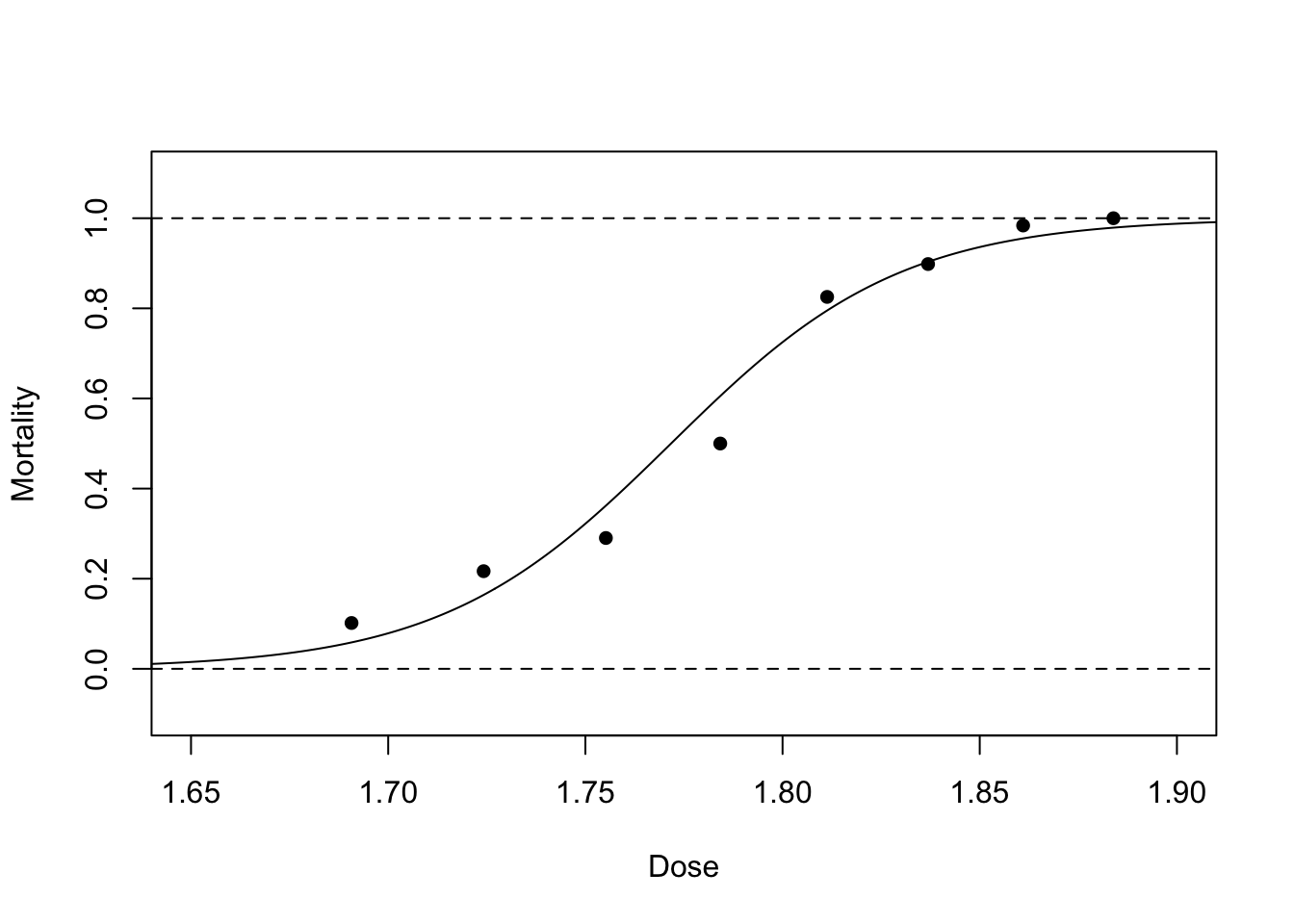
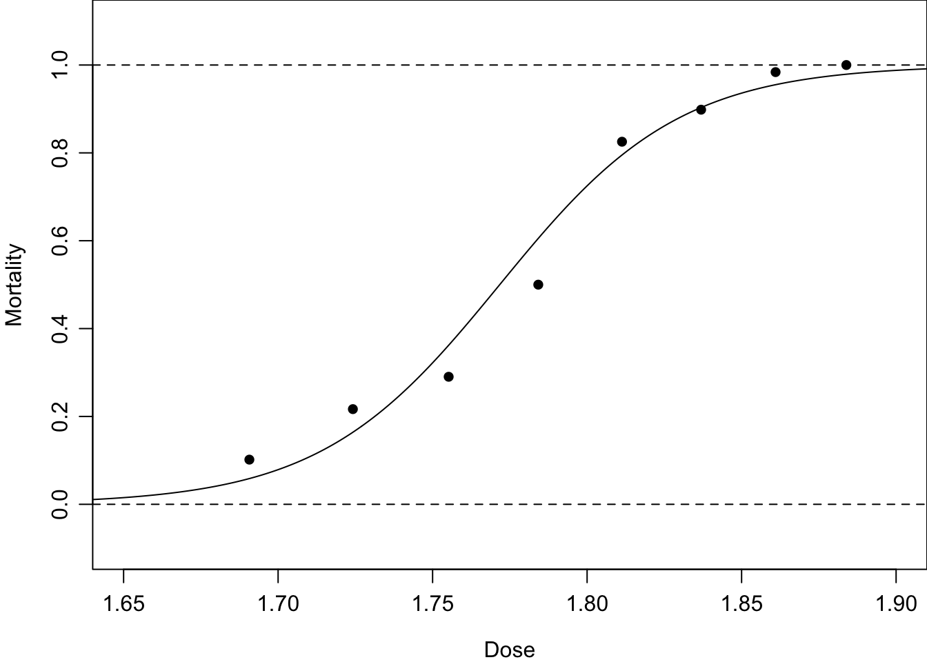
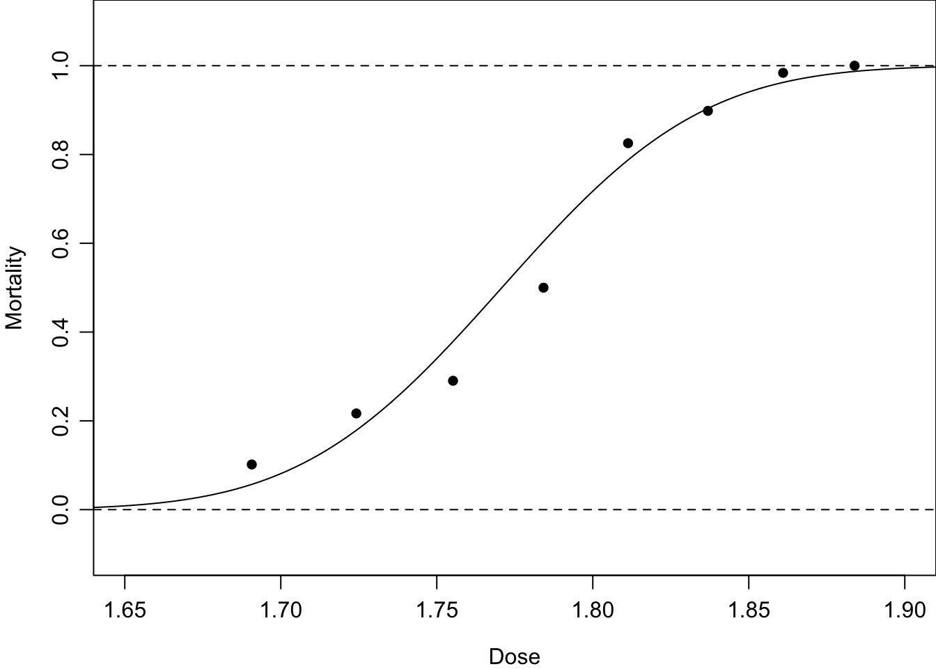
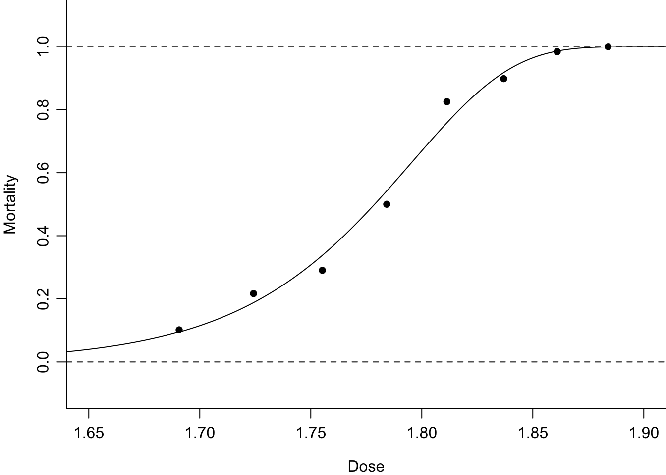
\tag{3.17}\]Figure 3.4 shows these link functions fitted to the beetle mortality data. The logit and probit links are very similar; the complementary log-log fits slightly better in the extremes; the cauchit link fits these data quite poorly in the extremes.
Figure 3.4: Dose–response curves fitted to the beetle mortality data with different choices of link function.
A mathematically and computationally convenient choice of link function \(g(\mu)\) can be constructed by setting \(\theta =\eta\), {#eq-g3} where \(\theta\) is the canonical parameter of the exponential family as defined in Equation 3.3. Then Equation 3.8 shows that the mean \(\mu\) is a function of \(\theta\) and therefore this indirectly provides a link between \(\mu\) and \(\eta\). Since \(\mu = b'(\theta)\), provided \(b'(\cdot)\) has an inverse, we may write \[
g(\mu) = \theta = (b')^{-1}(\mu).
\tag{3.18}\] The function produced from Equation 3.18 is called the canonical link function.
Proposition 3.2 For the canonical link function, \[
g'(\mu) = 1/b''(\theta).
\]
Proof: From Proposition 3.1, \(\mu = b'(\theta)\), so \(\text{d} \mu / \text{d} \theta = b''(\theta)\). From Equation 3.18, \(\text{d} \theta / \text{d} \mu = g'(\mu)\). Since \(\text{d} \theta /\text{d} \mu = (\text{d} \mu / \text{d} \theta)^{-1}\), we obtain \(g'(\mu) = 1/b''(\theta)\).
Example: Poisson canonical link function
For the Poisson distribution \(\text{Po}(\lambda)\), from Table 3.2, \(b(\theta) = e^\theta\) so \(b'(\theta) = e^\theta\). Applying Equation 3.18: \(g(\mu) = \log(\mu)\). Thus the canonical link for the Poisson is \(\log\).
Example: Normal canonical link function
For the Normal distribution \(N(\mu, \sigma^2)\), from Table 3.4, \(b(\theta) = \theta^2/2\) so \(b'(\theta) = \theta\). Applying Equation 3.18: \(g(\mu) = \mu\). Thus the canonical link for the Normal distribution is the identity function.
Table 3.6 summarises the canonical link functions for several distributions, showing that the canonical link maps the restricted range of \(\mu\) onto the whole real line for Normal, Poisson, and Binomial, but not for the Gamma.
Table 3.6: Canonical link functions and their ranges (\(\dagger\)binomial distribution with index \(m\) and mean \(\mu\); \(\ddagger\)gamma distribution with mean \(\mu\): see Exercises for details).
\(f(y)\)
Range of \(\mu\)
\(b(\theta)\)
\(\mu=b'(\theta)\)
Canonical link, \(g(\mu)\)
Range of \(\eta\)
Normal
\((-\infty, \infty)\)
\(\frac12 \theta^2\)
\(\theta\)
\(\mu\)
\((-\infty, \infty)\)
Poisson
\((0,\infty)\)
\(e^\theta\)
\(e^\theta\)
\(\log\mu\)
\((-\infty, \infty)\)
Binomial\(\dagger\)
\((0, m)\)
\(m\log(1+e^\theta)\)
\(m/(1+e^{-\theta})\)
\(\mbox{logit}(\mu/m)\)
\((-\infty, \infty)\)
Gamma\(\ddagger\)
\((0,\infty)\)
\(-\log (-\theta)\)
\(-\theta^{-1}\)
\(-\mu^{-1}\)
\((-\infty, 0)\)
Using the canonical link in the exponential family formula Equation 3.3 and taking \(n\) independent observations, the log-likelihood simplifies to \[
\log f(\mathbf{y}; \mathbf{X}, \boldsymbol{\beta},\phi) =
\frac{\sum_j \beta_j S_j - \sum_i b\left(\sum_j \beta_j x_{ij}\right)}
{\phi} + \sum_i c(y_i, \phi)
\tag{3.19}\] where \(S_j = \sum_{i=1}^n y_i x_{ij}\) are called sufficient statistics. Their appearance confers both theoretical and practical advantages.
Focus on link functions quiz
Test your knowledge recall and application to reinforce basic ideas and prepare for similar concepts later in the module.
If the response variable Y can take only positive values, then which of the following transformations would produce an unrestricted range?
If the range of the response variable Y is restricted to the interval (0,1), then which of the following transformations would produce an unrestricted range?
If response variable Y follows a normal distribution, then which of the following transformations would produce an unrestricted range?
If the range of the response variable Y is a percentage, then which of the following transformations would produce an unrestricted range?
If the response variable Y can take any real value, then which of the following transformations would produce an unrestricted range?
3.7 Exercises
3.1 Consider the beetle data again (see Table 1.1), but suppose that we had only been given the \(y\) values, that is the number killed, and misinformed that each came from a sample of size \(62\). Further, suppose that we did not know that different doses had been used. That is, we were given data: \(\mathbf{y}=\{6, 13, 18, 28, 52, 53, 61, 60\}\) and led to believe that the model \(Y\sim \mbox{Bin}(62,p)\) was appropriate. Use the given data to estimate \(p\). Then, calculate the fitted probabilities and superimpose them on a histogram of the data.
3.2 Verify that, in general, if \(q = 1/(1+e^{-x})\) then \(x = \log(q/(1-q))\) and then for the binomial distribution, \(Y\sim \mbox{Bin}(m,p)\), show that \[
-m\log(1-p)=m\log(1+e^\theta)
\] where \(\theta=\mbox{logit }p = \log(p/(1-p))\).
Each derivation requires algebraic rearrangement and simplification only.
3.3 Suppose that \(Y\) has a gamma distribution with parameters \(\alpha\) and \(\lambda\), that is \(Y\sim \mbox{Gamma}(\alpha, \lambda)\), with probability density function \[
f(y;\alpha, \lambda) = \frac{\lambda^\alpha y^{\alpha-1} e^{-\lambda y}}{\Gamma(\alpha)} \qquad y > 0; \alpha,\lambda>0.
\] Write this in the form of the exponential family and clearly identify \(\theta\), \(\phi\), \(b(\theta)\) and \(c(y,\phi)\) – as was done for the Poisson and binomial in Table 3.2 and Table 3.3.
Consider treating \(1/\alpha\) as a scale parameter and let \(\theta\) be a suitable function of \(\lambda\) and \(\alpha\).
3.4 Express the geometric distribution, \(Y\sim\mbox{Geom}(p), 0 < p <1\), with probability mass function \[
f(y) = (1 - p)^{y-1} p; \hspace{1cm} y = 1, 2, 3 \ldots
\] as an exponential family distribution.
Follow the same process as for the Poisson and binomial.
3.5 Prove Proposition 3.1 assuming that \(Y\) follows a discrete distribution. Use the proposition, starting from the given \(b(\theta)\), to verify the results for expectation and variance of the Poisson in Table 3.5 and then derive similar results for the binomial, \(Y\sim \mbox{Bin}(m,p)\).
Replace the integration in the continuous case by summation for the discrete case. For the binomial, find \(b(\theta)\) from Table 3.3 and then compute its first and second derivatives.
3.6 Use the properties of exponential families to find the expectation and variance of each of the geometric and gamma distributions considered above.
Use the results from Exercises 3.3 and 3.4, and apply Proposition 3.1.
3.7 Using Equation 3.18, verify the canonical link function, \(g(\mu)\), for the binomial and gamma distributions shown in Table 3.6.
Use the appropriate \(b'(\theta)\) and, using \(\mu=b'(\theta)\) and Equation 3.18, rearrange to find \(\theta\) and hence \(g(\mu)\).