16 Key Functions in Survival Analysis
16.1 The survival function
Let \(T > 0\) be a continuous random survival time with distribution function \(F(t) = \Prob(T \leq t)\) and density \(f(t) = F'(t)\).
\(S(t)\) is a non-increasing function with \(S(0) = 1\) and \(\lim_{t\to\infty} S(t) = 0\). For continuous \(T\), \[ S'(t) = -f(t) \qquad \Rightarrow \qquad f(t) = -S'(t). \]
16.2 The hazard function
Intuitively, \(h(t)\,\delta t \approx \Prob(\text{event in } [t, t+\delta t) \mid \text{survived to } t)\) for small \(\delta t\).
Using conditional probability and the definition of the density: \[ h(t) = \frac{f(t)}{S(t)} = -\frac{S'(t)}{S(t)} = -\frac{d}{dt}\log S(t). \]
The hazard can take any non-negative value. Unlike the density \(f(t)\), it is not a probability density and need not integrate to 1.
16.3 The cumulative hazard
Since \(h(t) = -d\log S(t)/dt\), integrating gives \[ H(t) = -\log S(t) \qquad \Longleftrightarrow \qquad S(t) = e^{-H(t)}. \]
This is one of the most important relationships in survival analysis. The three functions \(S(t)\), \(h(t)\), and \(H(t)\) each completely characterise the distribution of \(T\): knowing any one determines the others.
16.4 Relationship between the three functions
| Function | From \(S(t)\) | From \(h(t)\) |
|---|---|---|
| \(S(t)\) | — | \(e^{-H(t)}\) |
| \(f(t)\) | \(-S'(t)\) | \(h(t)e^{-H(t)}\) |
| \(h(t)\) | \(-S'(t)/S(t)\) | — |
| \(H(t)\) | \(-\log S(t)\) | \(\int_0^t h(s)\,ds\) |
16.5 Mean and median survival time
The mean survival time is \[ \E[T] = \int_0^\infty t\,f(t)\,dt = \int_0^\infty S(t)\,dt, \] where the second equality follows from integration by parts (under Assumption 2 of Chapter 15, \(\Prob(T < \infty) = 1\)).
The median survival time \(\mu_{1/2}\) satisfies \(S(\mu_{1/2}) = 0.5\), i.e., it is the time by which half the population has experienced the event. The median is often preferred over the mean in survival analysis because it is less sensitive to the (often unknown) tail behaviour of \(S(t)\).
For the exponential distribution: \(\E[T] = 1/\lambda\) and \(\mu_{1/2} = \log(2)/\lambda\).
More generally, the \(p\)th quantile satisfies \(S(t_p) = 1 - p\).
16.6 Empirical estimation (no censoring)
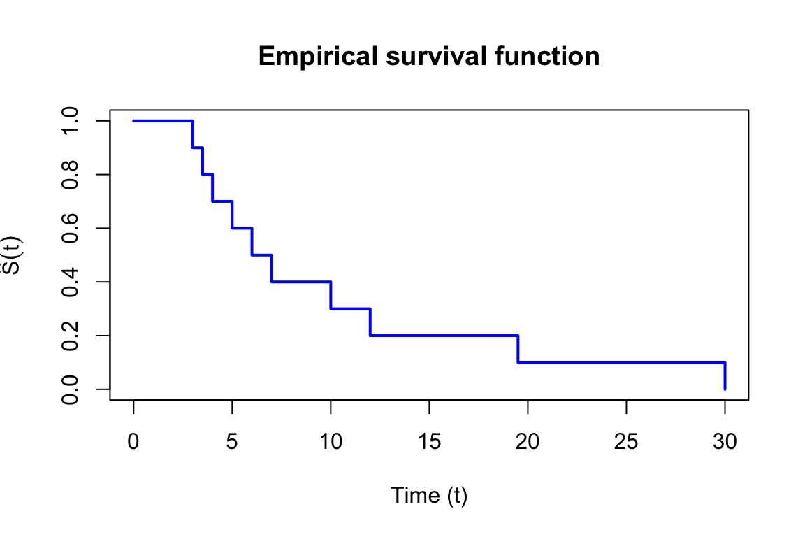
When data are uncensored, \(S(t)\) can be estimated by the empirical survival function \[ \widehat{S}(t) = \frac{\#\{i : t_i > t\}}{n}. \] This is an unbiased estimator: \(\E[\widehat{S}(t)] = S(t)\).
In R:
Code
library(survival)
t_obs <- c(3, 3.5, 4, 5, 6, 7, 10, 12, 19.5, 30)
model <- survfit(Surv(t_obs) ~ 1)
summary(model)
plot(model)
When data include censored observations, the empirical survival function is biased. The Kaplan–Meier estimator, introduced in Chapter 17, handles this correctly.
Exercises
16.1. Suppose a survival time \(T\) has hazard function \[h(t) = \frac{2}{t + 8}, \qquad t \geq 0.\]
- Find the cumulative hazard \(H(t)\).
- Hence write down the survival function \(S(t)\) and the probability density function \(f(t)\).
Recall \(H(t) = \int_0^t h(u)\,\mathrm{d}u\), \(S(t) = e^{-H(t)}\), and \(f(t) = h(t)S(t)\).
16.2. Continuing from Exercise 16.1 with \(S(t) = 64/(8+t)^2\).
- Find the mean survival time \(\E[T]\) using the formula \(\E[T] = \int_0^\infty S(t)\,\mathrm{d}t\).
- Find the median survival time \(t_{0.5}\), defined by \(S(t_{0.5}) = 0.5\).
For part (a), integrate \(64/(8+t)^2\) from 0 to \(\infty\). For part (b), solve \(64/(8+t_{0.5})^2 = 1/2\) for \(t_{0.5}\).