Parametric models (Chapters 17–22) require us to specify the shape of the baseline hazard \(h_0(t)\). In practice, we may not be confident in this choice, and a misspecified baseline can bias the estimated effects of the explanatory variables \(\hat{\bbeta}\).
In 1972, Sir David Cox proposed a semi-parametric approach that estimates \(\bbeta\) without specifying \(h_0(t)\) at all. The baseline hazard is treated as an unspecified nuisance function, and inference on \(\bbeta\) is based on a partial likelihood that eliminates \(h_0(t)\).
23.2 The Cox model
Definition: Cox proportional hazards model
\[
h(t \mid \mathbf{x}_i) = h_0(t)\exp(\bbeta^T\mathbf{x}_i),
\] where \(h_0(t) \geq 0\) is an unspecified baseline hazard function and \(\bbeta = (\beta_1, \ldots, \beta_p)^T\) are regression coefficients.
The explanatory-variable effects are the same as in the parametric PH model (Chapter 22). What is new is that \(h_0(t)\) is left completely unspecified.
23.3 Partial likelihood
Cox’s key insight was to construct a likelihood for \(\bbeta\) that does not involve \(h_0(t)\).
Let \(t_{(1)} < t_{(2)} < \cdots < t_{(r)}\) be the ordered event times (ties handled separately). At each event time \(t_{(j)}\), define the risk set\[
\mathcal{R}(t_{(j)}) = \{\text{individuals still at risk immediately before } t_{(j)}\}.
\]
Given that an event occurs at \(t_{(j)}\), the conditional probability that it is individual \(i_{(j)}\) who experiences the event (rather than any other at-risk individual) is \[
\frac{h_0(t_{(j)})\exp(\bbeta^T\mathbf{x}_{i_{(j)}})}
{\sum_{\ell \in \mathcal{R}(t_{(j)})} h_0(t_{(j)})\exp(\bbeta^T\mathbf{x}_\ell)}
= \frac{\exp(\bbeta^T\mathbf{x}_{i_{(j)}})}
{\sum_{\ell \in \mathcal{R}(t_{(j)})} \exp(\bbeta^T\mathbf{x}_\ell)}.
\]
The baseline hazard \(h_0(t_{(j)})\) cancels in the numerator and denominator.
Proof: See the supplementary notes proof_partial_likelihood.pdf for a full justification of this conditioning argument.
Definition: Partial likelihood
\[
L(\bbeta) = \prod_{j=1}^{r}
\frac{\exp(\bbeta^T\mathbf{x}_{(j)})}
{\displaystyle\sum_{\ell \in \mathcal{R}(t_{(j)})} \exp(\bbeta^T\mathbf{x}_\ell)},
\] where \(\mathbf{x}_{(j)}\) is the vector of explanatory variables for the individual who dies at time \(t_{(j)}\).
This can be written compactly as \[
L(\bbeta) = \prod_{i=1}^n \left[
\frac{\exp(\bbeta^T\mathbf{x}_i)}
{\sum_{\ell \in \mathcal{R}(t_i)} \exp(\bbeta^T\mathbf{x}_\ell)}
\right]^{\delta_i}.
\]
Only the \(\delta_i = 1\) terms contribute to the product.
The maximum partial likelihood estimator (MPLE)\(\hat{\bbeta}\) maximises Equation 23.1. Under regularity conditions, \(\hat{\bbeta}\) has the same asymptotic properties as an MLE: \[
\hat{\bbeta} \;\dot\sim\; \mathrm{N}_p\!\left(\bbeta,\; \mathcal{I}(\bbeta)^{-1}\right),
\] where \(\mathcal{I}(\bbeta) = -\partial^2\ell/\partial\bbeta\partial\bbeta^T\) is the observed information matrix.
23.5 Handling tied event times
The partial likelihood above assumes no ties. With ties, the most common approximation is Breslow’s approximation: \[
L(\bbeta) \approx \prod_{j=1}^r
\frac{\exp(\bbeta^T\mathbf{s}_{(j)})}
{\left(\displaystyle\sum_{\ell \in \mathcal{R}(t_{(j)})} \exp(\bbeta^T\mathbf{x}_\ell)\right)^{d_j}},
\] where \(d_j\) is the number of deaths at \(t_{(j)}\) and \(\mathbf{s}_{(j)}\) is the sum of the explanatory-variable vectors of those who die.
23.6 Manual calculation: coronavirus example
Example: Recovery from coronavirus
Six patients from two groups (Group I: lung condition; Group II: no lung condition) with event indicator and ordered recovery times:
Individual
Group
Time
Event
1
I
16
1
2
I
24
0 (censored)
3
I
28
0 (censored)
4
I
30
1
5
I
42
1
6
I
42
0 (censored)
7
II
6
1
8
II
10
0 (censored)
9
II
12
0 (censored)
10
II
30
0 (censored)
11
II
32
1
12
II
41
1
Let \(x_i = 0\) for Group I, \(x_i = 1\) for Group II. There are \(r = 6\) events at ordered times \(6, 16, 30, 32, 41, 42\).
The partial log-likelihood (ignoring the intercept, which does not identify \(\beta\)) is constructed term by term. By symmetry of the data, the MPLE turns out to be \(\hat\beta = \log 2 \approx 0.693\), giving hazard ratio \(\hat\psi = e^{\hat\beta} = 2\) for Group II relative to Group I: patients without a lung condition (Group II) recover at twice the rate of those with one (Group I) – equivalently, patients with a lung condition recover at half the rate of those without.
23.7 Cox model in R
Code
library(survival)# Basic Cox modelcox_fit <-coxph(Surv(t, delta) ~ x1 + x2, data = mydata,ties ="breslow")summary(cox_fit)# Output includes:# - Estimated coefficients beta_hat# - exp(coef): hazard ratios# - 95% CI for hazard ratios# - Wald, likelihood ratio, and score tests for overall significance
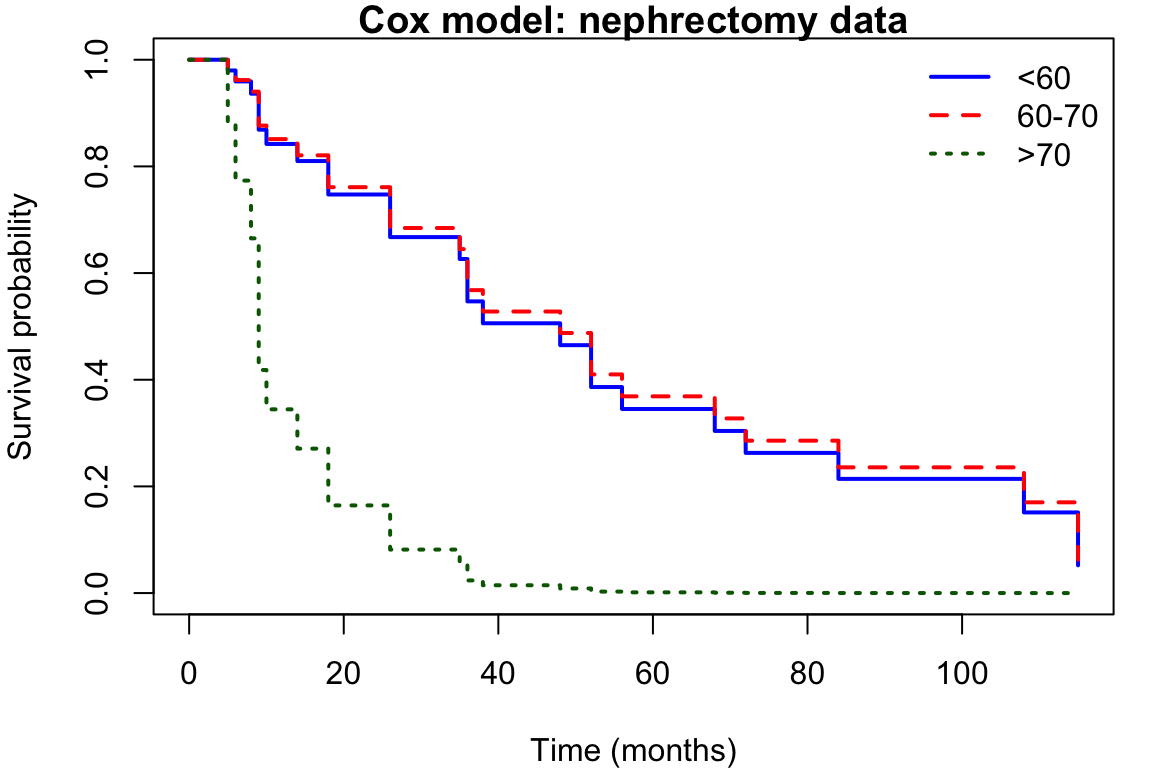
Figure 23.1: Baseline survival function estimated from the Cox model for the nephrectomy data. Separate curves are shown for patients under 60 (solid), 60–70 (dashed), and over 70 (dotted).
Code
library(survival)# Load datah <-read.table("https://www.richardpmann.com/MATH3701/Datasets/hypernephroma.dat", header =TRUE)h$age <-as.factor(h$age)levels(h$age) <-c("<60", "60-70", ">70")# Fit Cox model to nephrectomy patients onlyh2 <- h[h$nephrectomy ==1, ]cox_fit <-coxph(Surv(time, status) ~ age, data = h2, ties ="breslow")summary(cox_fit)
Exercises
23.1. A small clinical trial compares Drug A (\(x=0\)) and Drug B (\(x=1\)). Survival times (days) are:
Drug A: 2 (event), 4 (event), 9\(^*\) (censored), 12 (event)
Drug B: 3\(^*\) (censored), 5\(^*\) (censored), 8 (event), 14 (event)
The Cox proportional hazards model is \(h(t, x) = e^{\beta x} h_0(t)\).
Identify all event times and the corresponding risk sets. Hence write down the Cox partial likelihood \(L(\beta)\) and show that \[L(\beta) = C \cdot \frac{e^\beta}{(1+e^\beta)^4},\] stating the value of the constant \(C\).
At each event time \(t_{(j)}\), the partial likelihood contribution is \(e^{\beta x_{(j)}} / \sum_{k \in R(t_{(j)})} e^{\beta x_k}\), where \(x_{(j)}\) is the value of the explanatory variable for the subject who had the event. The risk set \(R(t_{(j)})\) contains all subjects with \(t_k \geq t_{(j)}\). Multiply contributions over all event times.
Find the maximum partial likelihood estimator \(\hat\beta\).
Differentiate \(\ell(\beta) = \log L(\beta)\) with respect to \(\beta\) and set to zero.
23.2. Continuing from Exercise 23.1 with \(\hat\beta = -\log 3\).
Compute the approximate variance of \(\hat\beta\) using the observed information \(-\ell''(\hat\beta)\).
Test \(H_0: \beta = 0\) (drugs equally effective) against a two-sided alternative at the 5% significance level using a Wald test.
Compute \(\ell''(\beta) = \mathrm{d}^2\ell/\mathrm{d}\beta^2\) from \(\ell'(\beta) = 1 - 4e^\beta/(1+e^\beta)\). Evaluate at \(\hat\beta\) and take the negative reciprocal for the variance. The Wald statistic is \(\hat\beta/\widehat{\mathrm{se}}(\hat\beta)\).