Recall from Chapter 15 that the observed data for each individual consist of a pair \((t_i, \delta_i)\) where \(t_i\) is the observed time and \(\delta_i = 1\) if the event was observed, \(\delta_i = 0\) if censored.
For an uncensored observation (\(\delta_i = 1\)), the event occurred at exactly time \(t_i\), contributing the density \(f(t_i)\) to the likelihood.
For a right-censored observation (\(\delta_i = 0\)), the individual survived beyond \(t_i\), contributing \(\Prob(T > t_i) = S(t_i)\).
Under the uninformative censoring assumption (Chapter 15), the full likelihood is
The second form has a natural interpretation: the survival function \(S(t_i)\) represents the probability of surviving until the observation time, and \(h(t_i)^{\delta_i}\) captures the (conditional) probability of the event occurring at that time if observed.
19.2 Exponential model: MLE derivation
For the exponential model with \(h(t) = \lambda\) and \(S(t) =
e^{-\lambda t}\), the log-likelihood is \[
\ell(\lambda) = \log L(\lambda) = \sum_{i=1}^n \left[\delta_i \log\lambda - \lambda t_i\right]
= r\log\lambda - \lambda v,
\] where \(r = \sum_i \delta_i\) is the number of observed events and \(v = \sum_i t_i\) is the total person-time.
This has an intuitive interpretation: the estimated hazard rate is the number of events per unit of total follow-up time.
Example: AVR data
For the AVR data (\(n = 5\), observed times 4, 5, 8, 10, 7; deaths at times 4, 8, 7): \[
r = 3, \qquad v = 4 + 5 + 8 + 10 + 7 = 34.
\] Therefore \(\hat\lambda = 3/34 \approx 0.088\) deaths per year. The estimated mean survival is \(1/\hat\lambda \approx 11.3\) years.
19.3 Weibull model: MLE
For the Weibull model with \(h(t) = \lambda\gamma t^{\gamma-1}\) and \(S(t) = e^{-\lambda t^\gamma}\), the log-likelihood is \[
\ell(\lambda, \gamma) = r\log(\lambda\gamma) + (\gamma-1)\sum_{i=1}^n \delta_i\log t_i
- \lambda \sum_{i=1}^n t_i^\gamma.
\]
There is no closed form for \(\hat\gamma\). The score equation \(\partial\ell/\partial\gamma = 0\) gives \[
\frac{1}{\gamma} + \frac{1}{r}\sum_{i=1}^n \delta_i\log t_i
- \frac{\sum_{i=1}^n t_i^\gamma \log t_i}{\sum_{i=1}^n t_i^\gamma} = 0.
\] This is solved numerically. Given \(\hat\gamma\), the profile MLE for \(\lambda\) is \[
\hat\lambda = \frac{r}{\sum_{i=1}^n t_i^{\hat\gamma}}.
\]
19.4 Fitting parametric models in R
Code
library(survival)# Load data (replace with actual dataset)# t = observed times# delta = event indicators (1 = event, 0 = censored)# Exponential modelfit_exp <-survreg(Surv(t, delta) ~1, dist ="exponential")# lambda_hat = exp(-coef(fit_exp))# Weibull modelfit_wei <-survreg(Surv(t, delta) ~1, dist ="weibull")gamma_hat <-1/ fit_wei$scalelambda_hat <-exp(-gamma_hat *coef(fit_wei)[1])cat("Weibull gamma:", gamma_hat, "\n")cat("Weibull lambda:", lambda_hat, "\n")# Log-likelihood values for model comparisonlogLik(fit_exp)logLik(fit_wei)
19.5 Model assessment via graphical checks
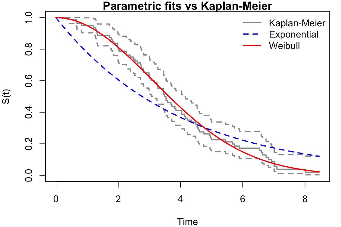
Having estimated the parameters, we should check the fit graphically by overlaying the fitted survival curve on the Kaplan–Meier estimate (see Chapter 17).
Figure 19.1: Kaplan–Meier estimate (step function) with fitted exponential (dashed) and Weibull (solid) curves for simulated data.
Exercises
19.1. Consider a survival model with hazard function \[h(t) = \lambda e^t, \qquad t \geq 0,\; \lambda > 0.\]
Find the survival function \(S(t)\).
Compute \(H(t) = \int_0^t h(u)\,\mathrm{d}u\) first, then use \(S(t) = e^{-H(t)}\).
19.2. Continuing from Exercise 19.1. Suppose we observe \(n\) independent individuals with survival times \(t_1, \ldots, t_n\), of which \(r\) are uncensored events (\(\delta_i = 1\)) and the rest are right-censored (\(\delta_i = 0\)).
Write the log-likelihood as \(\ell(\lambda) = \sum_i \delta_i \log f(t_i) + \sum_i (1-\delta_i)\log S(t_i)\). Substitute \(f(t) = h(t)S(t) = \lambda e^{t}e^{-\lambda(e^t-1)}\). Differentiate with respect to \(\lambda\) and set to zero.
Write down the log-likelihood \(\ell(\lambda)\) in terms of \(r\), \(\{t_i\}\), and \(\lambda\).
Derive the maximum likelihood estimator \(\hat\lambda\).