20 Parametric Two-Sample Comparison
20.1 Comparing two groups
Suppose individuals belong to one of two groups (e.g., two treatment arms, male/female, exposed/unexposed). We wish to test whether the survival distributions in the two groups are the same.
Let \(h_j(t)\) denote the hazard in group \(j\) (\(j = 1, 2\)). For each group, observe \((t_{ji}, \delta_{ji})\) for \(i = 1, \ldots, n_j\).
Define: - \(r_j = \sum_i \delta_{ji}\): number of events in group \(j\), - \(v_j = \sum_i t_{ji}\): total person-time in group \(j\).
20.2 Exponential two-sample model
Under the exponential model, \(h_j(t) = \lambda_j\) (constant), and the MLEs are \(\hat\lambda_j = r_j / v_j\) (from Chapter 19).
To compare the two groups, we use the hazard ratio \[ \psi = \frac{\lambda_2}{\lambda_1}, \] which is estimated by \(\hat\psi = \hat\lambda_2/\hat\lambda_1 = (r_2 v_1)/(r_1 v_2)\).
The log hazard ratio has an approximately normal distribution: \[ \log\hat\psi \;\dot\sim\; \mathrm{N}\!\left(\log\psi,\; \frac{1}{r_1} + \frac{1}{r_2}\right), \] giving a \(95\%\) confidence interval for \(\psi\): \[ \exp\!\left(\log\hat\psi \pm 1.96\sqrt{\frac{1}{r_1} + \frac{1}{r_2}}\right). \]
A likelihood ratio test of \(H_0: \psi = 1\) (equal hazards) uses \[ \Lambda = -2(\hat\ell_0 - \hat\ell_1) \;\dot\sim\; \chi^2_1 \] under \(H_0\), where \(\hat\ell_0\) is the maximised log-likelihood under \(\lambda_1 = \lambda_2\) and \(\hat\ell_1\) is the maximised log-likelihood with separate \(\lambda_j\).
20.3 Graphical check: the log-cumulative hazard
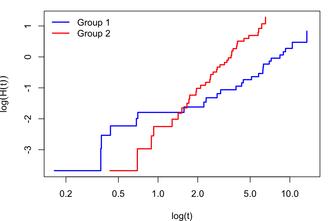
Before fitting any parametric model, it is important to check whether the chosen family is appropriate. For the exponential model: \[ H_j(t) = \lambda_j t \quad \Rightarrow \quad \log H_j(t) = \log\lambda_j + \log t. \]
A plot of \(\log\widehat{H}(t)\) against \(\log t\) should be linear with slope 1 for both groups. If the slopes differ from 1 but are equal to each other, a Weibull model with a common shape \(\gamma\) may be more appropriate.
20.4 Weibull two-sample model
For a common shape \(\gamma\) but different scales \(\lambda_1, \lambda_2\): \[ h_j(t) = \lambda_j \gamma t^{\gamma - 1}. \]
The hazard ratio \(\psi = \lambda_2/\lambda_1\) does not depend on \(t\) — this is the proportional hazards (PH) property, which is explored in detail in Chapter 21.
The MLEs of \(\lambda_j\) (given \(\hat\gamma\)) are \[ \hat\lambda_j = \frac{r_j}{\sum_i t_{ji}^{\hat\gamma}}, \] and \(\hat\gamma\) is obtained numerically by maximising the joint log-likelihood.
20.5 Fitting in R
Code
library(survival)

# Fit separate exponential models
fit1 <- survreg(Surv(t1, delta1) ~ 1, dist = "exponential")
fit2 <- survreg(Surv(t2, delta2) ~ 1, dist = "exponential")

# Or jointly using a group explanatory variable
# (see Chapter 22 for regression interpretation)
d <- data.frame(t = c(t1, t2), delta = c(d1, d2),
                group = c(rep(0, n1), rep(1, n2)))
fit_joint <- survreg(Surv(t, delta) ~ group, data = d,
                     dist = "exponential")
summary(fit_joint)
# coefficient on 'group' = -log(psi)
# (note: sign convention depends on parametrisation)
Exercises
20.1. A randomised trial compared two surgical approaches for a procedure, measuring operating time (minutes) until the surgeon achieved an adequate result. Times marked \(^*\) are right-censored at 120 minutes (procedure stopped without achieving the result):
- Group 1 (robot-assisted): 50, 51, 66\(^*\), 82, 92, 120\(^*\), 120\(^*\), 120\(^*\)
- Group 2 (traditional): 63, 65, 69, 69, 79, 82, 82, 120\(^*\)
Write R code to enter these data and produce a single plot showing the Kaplan–Meier survival curves for both groups, with appropriate labels, a legend, and 95% confidence intervals.
Based on the KM curves, which surgical approach achieves the adequate result sooner? Comment on the degree of overlap of the confidence intervals.
Use survfit(Surv(t, d) ~ group) and then plot() with col, lty, and legend(). A lower KM curve means events occur sooner; in this context that is the favourable outcome.
For the log-rank test, at each event time \(t_{(j)}\) compute \(E_{1j} = n_{1j} d_j / n_j\). The test statistic is \(U_L = \sum_j (O_{1j} - E_{1j})\) with variance \(\mathrm{Var}(U_L) = \sum_j n_{1j}n_{2j}d_j(n_j - d_j)/(n_j^2(n_j-1))\).
Carry out the normal-form log-rank test at the 10% significance level by hand, showing the calculation table.
State the chi-squared form of the test statistic and compare your conclusion with part (a). Verify your result using R.