Code
out = gam(y ~ s(x, fx=FALSE, k=6, sp=3.5))
out = gam(y ~ s(x, fx=FALSE, k=6))So far, we have considered the modelling of a response variable \(y\) in terms of a single explanatory variable \(x\). In particular, we have assumed that the form of this relationship is unknown but can be written as \[ y_i = f(x_i) + \epsilon_i,\qquad \epsilon_i\sim\text{N}(0,\sigma^2) \] where the \(\epsilon_i\) are i.i.d. and \(f(x)\) is assumed to be smooth. Given knot positions \(\{x_i,\; i=1,\dots,n\}\), we can estimate \(f(x)\) with a smoothing spline \(\hat{f}_\lambda(x)\) for given smoothing parameter \(\lambda\) and, further, we can estimate \(\lambda\) using ordinary or generalised cross-validation. This approach is in contrast to simple linear regression where \(y\) is expressed as a linear function of the explanatory variable, \(y_i=\alpha + \beta x_i +\epsilon_i\), which enforces a very inflexible relationship.
In this chapter, we generalise the modelling to describe the dependence of the response variable \(y\) on a set of explanatory variables \(\mathbf{x}=(x_1,x_2,\dots, x_p)\) where, conditionally on \(\mathbf{x}\), observation \(y\) has a distribution which is not necessarily normal.
Just as with a generalised linear model, the generalised additive model relates a continuous or discrete response variable \(Y\) to a set of explanatory variables \(\mathbf{x}=(x_1,x_2,\dots, x_p)\) and the model contains three parts:
Random part: The probability (mass or density) function of \(Y\) is assumed to belong to the two-parameter exponential family of distributions with parameters \(\theta\) and \(\phi\).
Systematic part: This is a non-linear predictor equation: \[ \eta = \sum_{j=1}^p f_j(x_j). \tag{14.1}\]
Link function: This is a one-to-one function providing the link between the predictor equation \(\eta\) and the mean \(\mu = \mathrm{E}[Y]\): \[ \eta = g(\mu), \quad \mbox{and} \quad \mu = g^{-1}(\eta) = h(\eta). \tag{14.2}\]
Here, \(g(\mu)\) is called the link function, and \(h(\eta)\) is called the inverse link function.
The spline theory in the previous chapters has assumed Gaussian (normally distributed) data and the identity link function. For non-Gaussian data and/or a non-identity link function, we replace the penalised least-squares criterion of Equation 12.2 with a penalised deviance: \[ R_{\nu}(f, \lambda, \boldsymbol{\beta}) = D({\mathbf y}, f,\boldsymbol{\beta}) + \lambda \, J_\nu(f), \tag{14.3}\] where \(D({\mathbf y}, f,\boldsymbol{\beta})\) is the deviance for the vector \(\mathbf{y}\) of observations modelled by a linear predictor that comprises a spline function \(f(x)\) of order \(\nu\) and possibly also main effects and interactions of explanatory variables. The penalised deviance is minimised with respect to the spline coefficients \(\mathbf{a}\), \(\mathbf{b}\) and regression parameters \(\boldsymbol{\beta}\), if any. Note that the fitted values for \(y\) are obtained by applying the inverse link function to the linear predictor \(f(x)\), for example the logistic function when the link is logit.
When there are several smooth terms of order \(\nu\) in the model, \({\mathbf f} = \{f_1,\dots,f_m\}\), each may be assigned its own roughness penalty \(\lambda_h\), and Equation 14.3 becomes \[ R_{\nu}(f_1,\dots,f_m, \lambda_1,\dots, \lambda_m, \boldsymbol{\beta}) = D({\mathbf y}, f_1,\dots,f_m, \boldsymbol{\beta}) + \sum_{h=1}^m \lambda_h J_\nu(f_h), \tag{14.4}\] or equivalently \[ R_{\nu}({\mathbf f}, {\boldsymbol \lambda}, \boldsymbol{\beta}) = D({\mathbf y}, {\mathbf f}, \boldsymbol{\beta}) + \sum_{h=1}^m \lambda_h J_\nu(f_h). \]
Fitting smoothing splines and GAMs is straightforward in practice using R. At the beginning of each R session, load the package mgcv, which makes available a set of routines written by Simon Wood of the University of Bristol.
The main command is gam, which fits a smoothing spline (or, more generally, a generalised additive model). The gam function is an extension to the glm command for fitting generalised linear models, allowing nonparametric functions of explanatory variables.
The syntax of the gam command is similar to that of glm. Suppose y is a vector of length n containing observations of a dependent variable and x is another vector of length n containing the corresponding explanatory variable values. Then each of the commands
out = gam(y ~ s(x, fx=FALSE, k=6, sp=3.5))
out = gam(y ~ s(x, fx=FALSE, k=6))fits a cubic smoothing spline to the dependent variable y. In the first version above, the user explicitly sets the smoothing parameter \(\lambda\) (denoted sp) to the value \(3.5\). In the second version, the optimal value of \(\lambda\) is chosen by the routine to minimise the Generalised Cross-Validation criterion, GCV. The notation s(x) means a smooth function (a cubic smoothing spline in this setting) of the explanatory variable x. Setting fx=FALSE in function s specifies that the dimensionality of the spline should be free. Parameter k of function s specifies the maximum dimensionality of the spline, and should be set according to the problem and data at hand since the default value will not be appropriate in general. For example, if x contains only 6 distinct values, then it would be appropriate to set k=6.
In each of the above examples, output from gam is stored in an object called out. This object contains several components of interest:
out$fitted.values is a vector of length n containing the fitted values of the smoothing spline at the data values.out$gcv.ubre contains the value of the GCV criterion.out$hat contains the diagonal values of the smoothing matrix, also called the hat matrix. The total degrees of freedom in the model (including the intercept term) is given by sum(out$hat).out$sp contains the smoothing parameter value.summary.gam(out) provides a summary of the smoothed model fit.anova.gam(out) provides an analysis of deviance for the model.Thus, if gam is called without an explicit choice of sp (as in the second example above), the output gives the optimal smoothing parameter value and the corresponding value of the GCV criterion.
To plot a smoothing spline:
predict.gam function to compute the cubic spline at these values.For example, suppose y is a vector of length 20 containing the responses at times \(1,\dots,20\).
# observation times
tt = 1:20
# compute a dense set of numbers between 0 and 21: 0, 0.1, ..., 21.0
ttnew = (0:210)/10
# compute predicted values at each of 0, 0.1, ..., 21.0
pred = predict.gam(out, newdata=list(tt=ttnew))
# plot the original data
plot(tt, y)
# superimpose the smoothing spline
lines(ttnew, pred)The textbook Elements of Statistical Learning, by Hastie, Tibshirani and Friedman (2nd Edn, 2011), refers to a case–control study of coronary heart disease (CHD) in South Africa. The data record the following variables for 462 males in a heart-disease high-risk region:
| Variable | Description |
|---|---|
tobacco |
cumulative tobacco consumption (kg) |
famhist |
family history of heart disease (Present, Absent) |
age |
age at onset of the disease (years) |
chd |
case–control status (1 = CHD; 0 = no CHD) |
hr <- read.table("https://www.richardpmann.com/MATH3701/Datasets/SAheart.txt", sep=",", head=TRUE, row.names=1)The dependent variable in our models will be chd. We model the CHD status of each individual as the result of a binary experiment (CHD or no CHD), using the Binomial distribution with index 1. The glm function allows such binary (0/1) dependent variables to be specified directly in the model formula.
We can examine CHD in relation to tobacco consumption, age and family history of heart disease, with the following R commands:
# make variables in dataframe hr directly available
attach(hr)

# fit a generalised linear model with chd as dependent variable
glm1 = glm(formula = 'chd ~ tobacco + age + famhist', family = 'binomial')
# examine the results
summary(glm1)
Call:
glm(formula = "chd ~ tobacco + age + famhist", family = "binomial")

Coefficients:
                Estimate Std. Error z value Pr(>|z|)
(Intercept)    -3.620593   0.444576  -8.144 3.83e-16 ***
tobacco         0.083004   0.025712   3.228  0.00125 **
age             0.048812   0.009452   5.164 2.42e-07 ***
famhistPresent  0.974791   0.220023   4.430 9.41e-06 ***
---
Signif. codes:  0 '***' 0.001 '**' 0.01 '*' 0.05 '.' 0.1 ' ' 1

(Dispersion parameter for binomial family taken to be 1)

    Null deviance: 596.11  on 461  degrees of freedom
Residual deviance: 495.39  on 458  degrees of freedom
AIC: 503.39

Number of Fisher Scoring iterations: 4
All variables in this model are statistically significant: disease is positively related to tobacco consumption, age and family history of heart disease. However, this model assumes that the logit of the probability of disease is linearly related to both tobacco consumption and age (logit being the default link for Binomial). We can explore more flexible tobacco-consumption and age trends with the following generalised additive model:
library(mgcv)Loading required package: nlmeThis is mgcv 1.9-1. For overview type 'help("mgcv-package")'.gam1 = gam(chd ~ s(tobacco, k=20) + s(age, k=20) + famhist,
family = 'binomial')
summary.gam(gam1)
Family: binomial
Link function: logit

Formula:
chd ~ s(tobacco, k = 20) + s(age, k = 20) + famhist

Parametric coefficients:
               Estimate Std. Error z value Pr(>|z|)
(Intercept)     -1.2379     0.1631  -7.592 3.15e-14 ***
famhistPresent   0.9628     0.2233   4.311 1.62e-05 ***
---
Signif. codes:  0 '***' 0.001 '**' 0.01 '*' 0.05 '.' 0.1 ' ' 1

Approximate significance of smooth terms:
             edf Ref.df Chi.sq  p-value
s(tobacco) 6.080  7.573  17.89   0.0179 *
s(age)     1.002  1.003  24.11 9.53e-07 ***
---
Signif. codes:  0 '***' 0.001 '**' 0.01 '*' 0.05 '.' 0.1 ' ' 1

R-sq.(adj) =  0.212   Deviance explained = 19.1%
UBRE = 0.083268  Scale est. = 1         n = 462
Here, the s function specifies a smooth (cubic spline) dependence. Parameter k of the s function specifies the maximum number of degrees of freedom allocated to this dependence. Setting k too small would restrict the set of basis functions used to construct the splines; setting k too large would increase the computational burden unnecessarily.
These results show that the fitted smoothing spline for tobacco consumption has an effective degrees of freedom (edf) of 6.080, while the dependence on age has edf of only 1.002, implying an almost linear age-dependence (a linear age term would have exactly 1 degree of freedom). See Section 13.5 for further details on the calculation of edf.
The significance of each smooth term is given by the \(p\)-value column in the table above. These \(p\)-values are computed from the \(\chi^2\) statistics in the previous column, whose approximate degrees of freedom are given in the column headed Ref.df. For example, the \(p\)-value of 0.0196 for s(tobacco) is computed by referring 17.62 to the \(\chi^2\) distribution on 7.573 degrees of freedom. Note that this compares the model above with the model which omits tobacco completely.
The following R code plots the fitted smooth functions of age and tobacco consumption:
# for larger axis labels
par(cex.lab=1.6)
# synthetic data for ages 15 to 65, no tobacco, no family history
newdat1 = data.frame(age = seq(from=15, to=65, by=0.1),
                     tobacco = 0, famhist = "Absent")
# predict logit probability of CHD
pred1 = predict.gam(gam1, newdata=newdat1)
# plot
plot(newdat1$age, pred1,
     xlab = "Age",
     ylab = "Predicted logit probability of CHD",
     type = "l")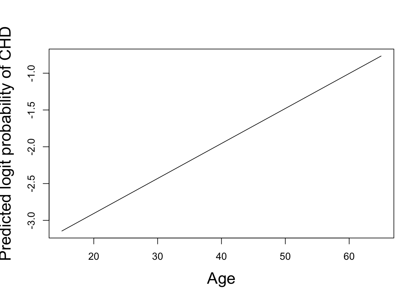
# synthetic data for age 40, tobacco from 0 to 32 kg, no family history
newdat2 = data.frame(age = 40,
                     tobacco = seq(from=0, to=32, by=0.1),
                     famhist = "Absent")
# predict logit probability of CHD
pred2 = predict.gam(gam1, newdata=newdat2)
# plot
plot(newdat2$tobacco, pred2,
     xlab = "Tobacco consumption",
     ylab = "Predicted logit probability of CHD",
     type = "l")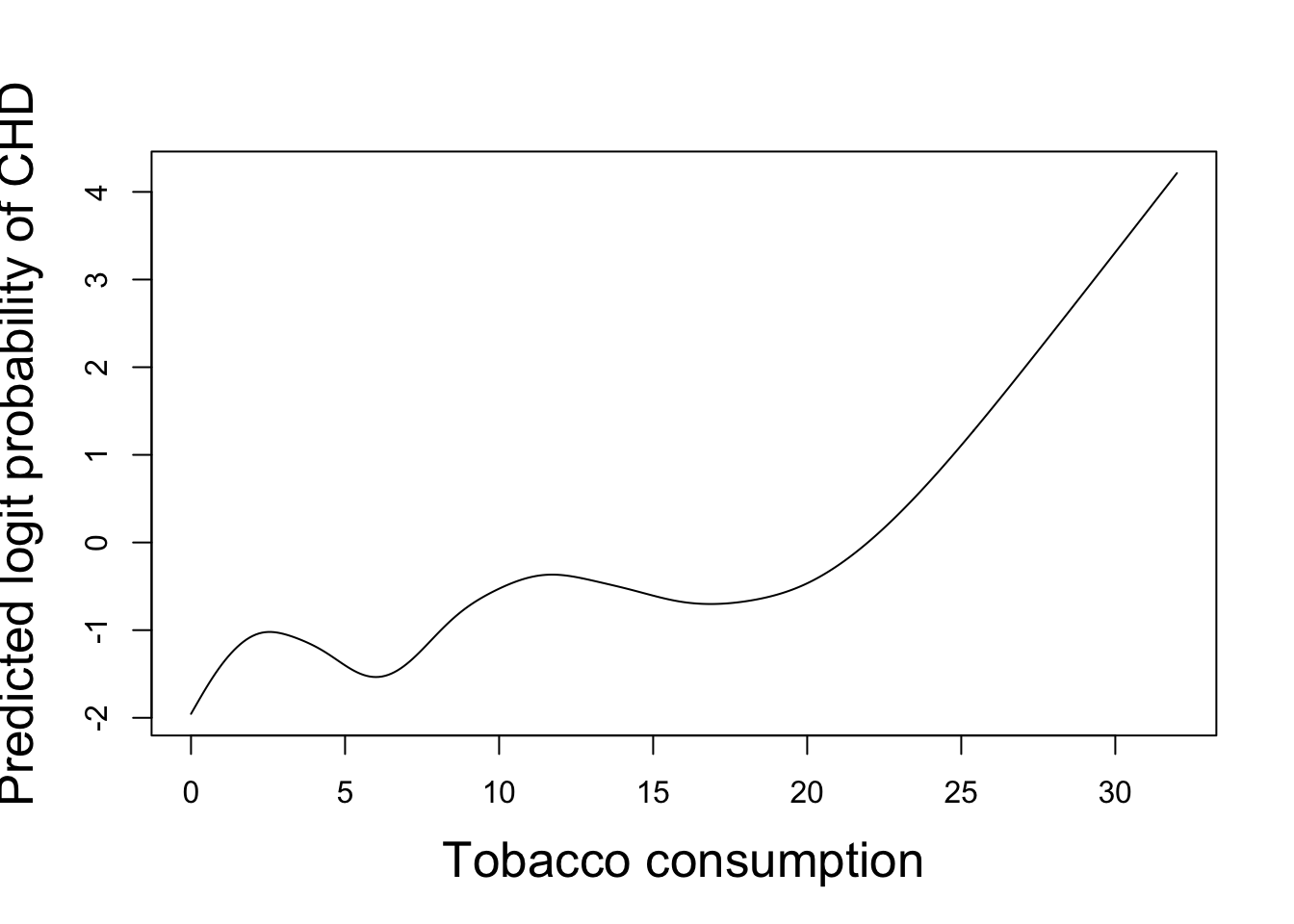
The predicted dependence of the logit probability of CHD on smooth functions of age and tobacco consumption is shown above. We see an almost linear predicted age-dependence, in agreement with its edf. The curious predicted dependence on tobacco consumption may be explained by other factors correlated with tobacco consumption.
14.1 Using the South Africa heart disease data (https://www.richardpmann.com/MATH3701/Datasets/SAheart.txt), fit a GAM that includes smooth terms for all continuous predictors (tobacco, alcohol, obesity, sbp, ldl, adiposity, typea) along with famhist as a parametric term and chd as the binary response.
Report the edf for each smooth term. Which predictors show evidence of non-linearity?
Fit a second model with the smooth term for alcohol removed (keeping all other smooth terms and famhist). This model is nested within the full model from part (a). Test whether alcohol should be retained by computing the change in deviance and the change in degrees of freedom between the two models, and comparing this to the appropriate \(\chi^2\) reference distribution (as in Section 4.3). What do you conclude?
Compare the full model and the model without alcohol using their GCV scores. Does this agree with your conclusion from the deviance test in (b)?
Repeat parts (b) and (c), but this time removing the smooth term for tobacco instead of alcohol.
Compare your conclusions for alcohol and tobacco. Do the deviance test and the GCV comparison agree with each other in both cases? What does this tell you about the roles of these two predictors in the model?
Fit the full model with gam(chd ~ s(tobacco,k=10) + s(alcohol,k=10) + ... + famhist, family='binomial'). An edf close to 1 suggests the smooth term is approximately linear and could be replaced by a parametric linear term. For (b) and (d), fit the reduced model with the relevant s(...) term simply omitted from the formula; the two models’ deviances are model$deviance, and a reasonable degrees-of-freedom for the test is the difference in their total edf (sum(model$edf)), used as in \(D_1-D_2\sim\chi^2_{r_2-r_1}\) even though this edf difference need not be an integer. For (c) and (d), compare model$gcv.ubre for the two models.
14.2 Using the mcycle data set from the MASS package (accelerometer readings from a motorcycle crash test), fit a GAM with times as the explanatory variable and accel as the response.
Fit the model using the gam function, allowing the GCV-minimising smoothing parameter to be automatically selected, and report the estimated edf.
Plot the fitted smooth function with its 95% confidence band.
Compare the GCV-optimal fit with fits obtained using a fixed smoothing parameter (sp) of \(10^{-4}\) and \(10^2\) (use the option sp = 1e-4 or sp = 1e2 in the gam function). Comment on the differences.
Use library(MASS); data(mcycle) to load the data. For part (b), use plot.gam(out, shade=TRUE).